pcalc.presence
A Presence is a foundational concept in the presence calculus and this module includes all the concepts for modeling presence and the API to work with them.
Formally, a presence may represented as a 5-tuple:
$$ p = (e, b, t_0, t_1, m) $$
where:
- $e \in E \subseteq D$ is an element (thing) in the domain $D$,
- $b \in B \subseteq D$ is the boundary (place) in the domain $D$,
- $[t_0, t_1)$ is the half-open interval of presence in time.
- $m \in R$ is called the mass of the presence.
A presence can be viewed as a function:
$$ P: E \times B \times \overline{\mathbb{R}} \times \overline{\mathbb{R}} \to \mathbb{R} $$
where
- $P(e, b, t_0, t_1) = m \gt 0 $ if $e$ is present in $b$ during $[t_0, t_1)$
- $P(e, b, t_0, t_1) = 0 $ otherwise
When $m \in \{ 0,1 \} $ we get the simplest form of presence: a binary assertion. This is a statement that an element was present in a boundary for a continuous time interval (with mass = 1).
Presence mass is core concept that will be described in more detail shortly - for now, it is sufficient to think of it as a value or weight attached to a presence assertion that is derived from some function on the underlying domain that must be "measurable" in a precise mathematical sense.
The key thing is that the machinery of the presence calculus lets you work identically with binaru presences which are much more intutive and easy to understand, and presences derived on arbitrary measures. This generality gives us a great deal of power on reasoning about logical, desterministic/stochastic, linear/non-linear and complex adaptive systems using exactly the same set of tools.
Presence onset and reset
$t_0$ is called the onset time of the presence—the instant at which the presence transitions from zero to non-zero mass. $t_1$ is called the reset time — the instant at which the presence transitions back to zero.
We will say the presence is active over the half-open interval $[t_0, t_1)$ (meaning it includes $t_0$ but excludes $t_1$).
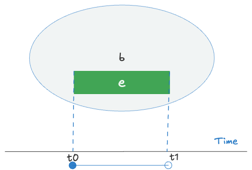
This diagram illustrates a presence assertion over a half-open interval $[t_0, t_1)$, where element $e$ is continuously present in boundary $b$ starting at $t_0$ (included) and ending just before $t_1$ (excluded).
The Open World Assumption
The time interval $[t_0, t_1)$ is defined over the extended reals $\overline{\mathbb{R}}$: the real line $\mathbb{R}$ extended with the symbols $-\infty$ and $+\infty$.
This reflects the presence calculus's open world assumption, which permits intervals that extend indefinitely into the past or future. A presence with $t_0 = -\infty$ represents a presence whose beginning is unknown, and $t_1 = +\infty$ represents a presence whose end is unknown.
Presences with both start and end unknown are valid and represent eternal presences. Many of the most interesting questions in the presence calculus involve reasoning about the dynamics of a domain under the epistemic uncertainty introduced by such presences.
Presence Assertions
A Presence Assertion is an assertion about the existence of a presence from the standpoint of a specific observer at a specific time.
A presence assertion is thus a seven-tuple $(e, b, t_0, t_1, m, o, t_2)$ where:
- $(e, b, t_0, t_1, m)$ is the presence being asserted,
- $o \in O \subseteq D$ is the observer (a domain entity), and
- $t_2 \in \overline{\mathbb{R}}$ is the assertion time.
Both observer and assertion time may themselves be unknown, and together they reflect the epistemic provenance of the assertion.
Given our open world assumptions, we assume by default that we are reasoning about dynamic sets of presences that reflect observations by various observers on the underlying domain. Presence assertions may be added or removed from this set, which in turn changes what we can say about the state of the domain. We assume (by construction, if necessary) that observers are part of the domain $D$.
For example, learning the reset time of a presence—when it was previously unknown—allows us to replace the old assertion with a new one that reflects greater epistemic certainty about the domain state. A new assertion may update the onset or reset time based on new information from different observers (e.g., sensor disagreements), reflecting the evolving nature of knowledge in an open world.
At any point in time, we are reasoning about a known subset of the domain's history, and potentially even making assertions about the future (estimates, forecasts, etc., which can also be modeled as presence assertions), each with its own epistemic status.
It is crucial to note that the presence calculus treats presence assertions as axiomatic: it does not question or infer their validity, nor does it make decisions based on provenance. However, the provenance of assertions may be used to reason about the reliability or implications of the conclusions reached via the machinery of the calculus.
For example, suppose in a traffic domain we observe that a vehicle (the element) crossed the 1-mile marker at 11:00 AM and the 2-mile marker at 11:10 AM. If we assert that the vehicle was continuously present (i.e., within the boundary between those markers) during the interval [11:00, 11:11), that assertion depends on domain-level assumptions—such as continuity of motion, absence of detours, or the nonexistence of teleportation.
In a different domain—for example, one in which a wormhole allows instantaneous travel between Mars and mile 1.6—such an assertion might be invalid.
The presence calculus does not attempt to resolve or validate such assumptions. It simply assumes that all presence assertions are logically valid according to domain semantics and proceeds to compute their consequences using the machinery of the calculus.
The key requirement though, is that the presence mass must be well defined. This brings us to the concept of a domain Signal over which presences are defined and asserted.
Domain Signals and Presence Mass
A Domain Signal is any function that varies over time and is associated with elements and boundaries in a given domain $D$. It may represent activity, value, demand, or any other observable quantity relevant to the system.
Let $$ F : (e, b, t) \to \mathbb{R}_{\geq 0} $$ be a function that assigns a non-negative value to each element–boundary–time triple. This is the general form of a domain signal in the Presence Calculus.
For the signal to be meaningful in the Presence Calculus, it must be measurable - that is, it must define a quantity that can be accumulated over time.
Measure theory and the Lebesgue measure provide the standard mathematical language to model such functions. In particular, the Lebesgue integral of the signal defines the presence mass: the total contribution it makes over a continuous time interval.
Integrability is the core requirement here—if a signal is Lebesgue integrable over an interval $[t_0, t_1)$, then its presence mass is well-defined and finite. This makes it possible to work with irregular, discontinuous, or sparse signals while still reasoning rigorously about accumulation and duration.
Given $(e, b, t_0, t_1)$, the presence mass is given by: $$ \mu_{e,b} = \int_{t_0}^{t_1} F(e, b, t)\, dt $$
This integral defines how much presence is accumulated over the interval for the given element–boundary pair, combining both the values of the function and how they are distributed over time.
This is not a particularly restrictive condition: the class of Lebesgue integrable functions is broad and includes most real-world signals encountered in practice. However, insisting that we use the Lebesgue integral to define mass over an interval (as opposed to, say, a statistical average) has meaningful consequences when modeling discontinuous signals. It ensures that the resulting "mass" retains its intended semantics as a presence measure, even as we apply more complex algebraic and topological operations to sets of presence assertions.
The Presence Calculus builds on this foundation, treating presence assertions as time-localized signals whose mass can be integrated, compared, and composed across boundaries.
In addition to integrability, a key property of a Lebesgue measure is that it must be finitely additive—that is, we must be able to compute sums over unions and intersections of sets of intervals.
Time as Topology
This brings us to a fundamental property of presences—and the key distinction between presences and point-in-time events: the continuity of presence gives us a natural and mathematically precise way to define a topology of presence over the extended real line $\overline{\mathbb{R}}$.
Each presence defines a basic open set in this topology, corresponding to its half-open interval $[t_0, t_1) \subset \overline{\mathbb{R}}.$ The collection of all such intervals forms a basis for a topology over time, using the standard technique from point-set topology of generating a topology from a basis of open sets. See BasisTopology for details.
This topological structure plays an important role in ensuring that presence mass is well-behaved under composition: it allows us to combine, intersect, and partition presences in ways that naturally satisfy the finite additivity conditions required for presence mass to behave like a Lebesgue measure.
This means that presence assertions allow us to reason about concepts such as nearness, overlap, continuity, and structure of presence in time— that is, how domain entities relate across time with mathematical precision.
It also allows us to compute sums, rates, averages, and other quantities across presences with well-defined semantics. This may seem like a technical detail, but it is essential: it allows us to handle sparse, discontinuous, bursty, or qualitative data with the same rigor as continuous signals.
The consequences of reasoning with presence assertions are temporal and topological: they give rise to notions of proximity, flow, and co-presence in time that reveal the shape, connectedness, and dynamics of the domain in mathematically precise ways.
With presence assertions, we can reason about patterns such as:
- elements that tend to be present together (co-presence),
- transitions between boundaries,
- regions of concentrated or evolving presence, and
- causal relationships between presences.
Furthermore, the Presence Calculus introduces certain topological invariants (see PresenceInvariant) that express general laws of conservation of presence mass.
This provides the foundational structure for reasoning about the dynamics and causality of presence in a domain.
Presence API
This module defines the data structure and associated methods for Presence, and serves as the canonical representation of presence assertions and their topological primitives in the presence calculus
Note: When interfacing with external systems that operate in wallclock time you will need to convert between timestamps and dates and floating point numbers when constructing presence assertions.
The TimeModel class (pcalc.time_model.TimeModel) is provided for this purpose.
  1# -*- coding: utf-8 -*-
  2# Copyright (c) 2025 Krishna Kumar
  3# SPDX-License-Identifier: MIT
  4"""
  5A *Presence* is a foundational concept in the presence calculus and this module
  6includes all the concepts for modeling presence and the API to work with them.
  7
  8Formally, a presence may represented as a 5-tuple:
  9
 10$$
 11p = (e, b, t_0, t_1, m)
 12$$
 13
 14where:
 15- $e \in E \subseteq D$ is an element (thing) in the domain $D$,
 16- $b \in B \subseteq D$ is the boundary (place) in the domain $D$,
 17- $[t_0, t_1)$ is the half-open interval of presence in time.
 18- $m \in R$ is called the
 19<em>mass</em> of the presence.
 20
 21A presence can be viewed as a function:
 22
 23$$
 24P: E \\times B \\times \\overline{\\mathbb{R}} \\times \\overline{\\mathbb{R}} \\to \\mathbb{R}
 25$$
 26
 27
 28where
 29
 30
 31- $P(e, b, t_0, t_1) = m \gt 0 $  if $e$ is present in $b$ during $[t_0, t_1)$
 32- $P(e, b, t_0, t_1) = 0 $    otherwise
 33
 34
 35When $m \in
 36\\\\{ 0,1 \\\\} $ we get the simplest form of presence: a binary assertion. This is a statement that an element was
 37present in a boundary for a continuous time interval (with mass = 1).
 38
 39Presence *mass* is core concept that
 40will be described in more detail shortly - for now, it is sufficient to think of it as a value or weight attached to
 41a presence assertion that is derived from some function on the underlying domain that must be "measurable" in a precise
 42mathematical sense.
 43
 44The key thing is that the machinery of the presence calculus lets you work identically with binaru presences which are much more
 45intutive and easy to understand, and presences derived on arbitrary measures. This generality gives us a great deal of power
 46on reasoning about logical, desterministic/stochastic, linear/non-linear and complex adaptive systems using exactly the
 47same set of tools.
 48
 49### Presence onset and reset
 50
 51$t_0$ is called the <em>onset time</em> of the presence—the instant at which the
 52presence transitions from zero to non-zero mass. $t_1$ is called the *reset time* —
 53the instant at which the presence transitions back to zero.
 54
 55We will say the presence is *active*
 56over the half-open interval $[t_0, t_1)$ (meaning it
 57includes $t_0$ but excludes $t_1$).
 58
 59<div style="text-align: center; margin: 2em 0;">
 60  <img src="../../assets/pcalc/half_open_presence.png" width="400px" />
 61  <div style="font-size: 0.9em; color: #555; margin-top: 0.5em;">
 62    Figure: A presence interval $[t_0, t_1)$ with $t_0$ included (●) and
 63    $t_1$ excluded (○).
 64  </div>
 65</div>
 66
 67This diagram illustrates a presence assertion over a half-open interval
 68$[t_0, t_1)$, where element $e$ is continuously present in boundary $b$
 69starting at $t_0$ (included) and ending just before $t_1$ (excluded).
 70
 71
 72
 73### The Open World Assumption
 74
 75The time interval $[t_0, t_1)$ is defined over the <em>extended</em> reals
 76$\overline{\mathbb{R}}$: the real line $\mathbb{R}$ extended with the symbols
 77$-\infty$ and $+\infty$.
 78
 79This reflects the presence calculus's open world assumption, which permits
 80intervals that extend indefinitely into the past or future. A presence with
 81$t_0 = -\infty$ represents a presence whose beginning is unknown, and
 82$t_1 = +\infty$ represents a presence whose end is unknown.
 83
 84Presences with both start and end unknown are valid and represent eternal
 85presences. Many of the most interesting questions in the presence calculus
 86involve reasoning about the dynamics of a domain under the epistemic
 87uncertainty introduced by such presences.
 88
 89---
 90### Presence Assertions
 91
 92A Presence Assertion is an assertion about the existence of a presence from
 93the standpoint of a specific observer at a specific time.
 94
 95A presence assertion is thus a seven-tuple
 96$(e, b, t_0, t_1, m, o, t_2)$ where:
 97
 98- $(e, b, t_0, t_1, m)$ is the presence being asserted,
 99- $o \in O \subseteq D$ is the observer (a domain entity), and
100- $t_2 \in \overline{\mathbb{R}}$ is the assertion time.
101
102Both observer and assertion time may themselves be unknown, and together
103they reflect the epistemic *provenance* of the assertion.
104
105Given our open world assumptions, we assume by default that we are reasoning
106about *dynamic* sets of presences that reflect observations by various observers
107on the underlying domain. Presence assertions may be added or removed
108from this set, which in turn changes what we can say about the
109state of the domain. We assume (by construction, if necessary) that observers
110are part of the domain $D$.
111
112For example, learning the reset time of a presence—when it was previously
113unknown—allows us to replace the old assertion with a new one that reflects
114greater epistemic certainty about the domain state. A new assertion may update
115the onset or reset time based on new information from different observers
116(e.g., sensor disagreements), reflecting the evolving nature of knowledge in
117an open world.
118
119At any point in time, we are reasoning about a known subset of the domain's
120history, and potentially even making assertions about the *future*
121(estimates, forecasts, etc., which can also be modeled as presence assertions),
122each with its own epistemic status.
123
124It is crucial to note that the presence calculus treats presence assertions as
125*axiomatic*: it does not question or infer their validity, nor does it make
126decisions based on provenance. However, the provenance of assertions may be
127used to reason about the reliability or implications of the conclusions reached
128via the machinery of the calculus.
129
130For example, suppose in a traffic domain we observe that a vehicle (the
131element) crossed the 1-mile marker at 11:00 AM and the 2-mile marker at
13211:10 AM. If we assert that the vehicle was continuously present (i.e.,
133within the boundary between those markers) during the interval [11:00, 11:11),
134that assertion depends on domain-level assumptions—such as continuity of
135motion, absence of detours, or the nonexistence of teleportation.
136
137In a different domain—for example, one in which a wormhole allows
138instantaneous travel between Mars and mile 1.6—such an assertion might be
139invalid.
140
141The presence calculus does *not* attempt to resolve or validate such
142assumptions. It simply assumes that all presence assertions are logically
143valid according to domain semantics and proceeds to compute their
144consequences using the machinery of the calculus.
145
146The key requirement though, is that the *presence mass* must be well defined.
147This brings us to the concept of a domain Signal over which presences are defined
148and asserted.
149
150### Domain Signals and Presence Mass
151
152A Domain Signal is any function that varies over time and is associated with
153elements and boundaries in a given domain $D$. It may represent activity,
154value, demand, or any other observable quantity relevant to the system.
155
156Let
157$$
158F : (e, b, t) \\to \\mathbb{R}_{\\geq 0}
159$$
160be a function that assigns a non-negative value to each element–boundary–time triple.
161This is the general form of a domain signal in the Presence Calculus.
162
163For the signal to be meaningful in the Presence Calculus, it must be *measurable* -
164that is, it must define a quantity that can be accumulated over time.
165
166*Measure theory* and the *Lebesgue measure* provide the standard mathematical language
167to model such functions. In particular, the *Lebesgue integral* of the signal
168defines the presence mass: the total contribution it makes over
169a continuous time interval.
170
171Integrability is the core requirement here—if a
172signal is Lebesgue integrable over an interval $[t_0, t_1)$, then its
173presence mass is well-defined and finite. This makes it possible to work with
174irregular, discontinuous, or sparse signals while still reasoning rigorously
175about accumulation and duration.
176
177Given $(e, b, t_0, t_1)$, the presence mass is given by:
178$$
179\\mu_{e,b} = \\int_{t_0}^{t_1} F(e, b, t)\\, dt
180$$
181
182This integral defines how much presence is accumulated over the interval for
183the given element–boundary pair, combining both the values of the function
184and how they are distributed over time.
185
186This is not a particularly restrictive condition: the class of Lebesgue integrable
187functions is broad and includes most real-world signals encountered in practice.
188However, insisting that we use the Lebesgue integral to define mass over an interval
189(as opposed to, say, a statistical average) has meaningful consequences when modeling
190discontinuous signals. It ensures that the resulting "mass" retains its intended semantics
191as a presence measure, even as we apply more complex algebraic and topological operations
192to sets of presence assertions.
193
194The Presence Calculus builds on this foundation, treating presence assertions
195as time-localized signals whose mass can be integrated, compared, and composed
196across boundaries.
197
198In addition to integrability, a key property of a Lebesgue measure is that it
199must be finitely additive—that is, we must be able to compute sums over
200unions and intersections of sets of intervals.
201
202### Time as Topology
203
204This brings us to a fundamental property of presences—and the key distinction
205between presences and point-in-time events: the continuity of presence gives us
206a natural and mathematically precise way to define a *topology* of presence
207over the extended real line $\overline{\\mathbb{R}}$.
208
209Each presence defines a basic open set in this topology, corresponding to its
210half-open interval $[t_0, t_1) \\subset \\overline{\\mathbb{R}}.$ The collection of
211all such intervals forms a basis for a topology over time, using the standard
212technique from point-set topology of generating a topology from a basis of
213open sets. See [BasisTopology](./basis_topology.html) for details.
214
215This topological structure plays an
216important role in ensuring that presence mass is well-behaved under composition:
217it allows us to combine, intersect, and partition presences in ways that
218naturally satisfy the finite additivity conditions required for presence mass
219to behave like a Lebesgue measure.
220
221This means that presence assertions allow us to reason about concepts such as
222*nearness*, *overlap*, *continuity*, and *structure* of presence in time—
223that is, how domain entities relate across time with mathematical precision.
224
225It also allows us to compute sums, rates, averages, and other quantities across
226presences with well-defined semantics. This may seem like a technical detail,
227but it is essential: it allows us to handle sparse, discontinuous, bursty, or
228qualitative data with the same rigor as continuous signals.
229
230The consequences of reasoning with presence assertions are *temporal* and *topological*:
231they give rise to notions of proximity, flow, and co-presence in time that reveal
232the shape, connectedness, and dynamics of the domain in mathematically precise ways.
233
234With presence assertions, we can reason about patterns such as:
235- elements that tend to be present together (*co-presence*),
236- transitions between boundaries,
237- regions of concentrated or evolving presence, and
238- causal relationships between presences.
239
240Furthermore, the Presence Calculus introduces certain topological invariants
241(see [PresenceInvariant](./presence_invariant_discrete.html)) that express
242general *laws of conservation of presence mass*.
243
244This provides the foundational structure for reasoning about the *dynamics*
245and *causality* of presence in a domain.
246
247---
248
249## Presence API
250
251This module defines the data structure and associated methods for Presence,
252and serves as the canonical representation of presence assertions and their topological
253 primitives in the
254presence calculus
255
256Note: When interfacing with external systems that operate in wallclock time you will need to
257convert between timestamps and dates and floating point numbers when constructing presence assertions.
258
259The [TimeModel](./time_model.html) class (`pcalc.time_model.TimeModel`) is provided for this purpose.
260
261---
262"""
263
264from __future__ import annotations
265from typing import Optional, Protocol, runtime_checkable
266
267from dataclasses import dataclass
268from typing import Optional, Callable
269
270from .entity import EntityProtocol
271
272
273PresenceFunction = Callable[[EntityProtocol, EntityProtocol, float], float]
274# Presence functions and Presence Protocols
275"""
276A `PresenceFunction` $f$ is a time-varying function represented as a callable of the form:
277
278```python
279(e: EntityProtocol, b: EntityProtocol, t: float) -> float
280```
281
282It returns a real-valued signal that is non-zero only when $t$ falls within some half open
283interval $[t_s, t_e)$
284
285Presence functions must satisfy the following property:
286
287- For some half-open interval $[t_s, t_e) in \overline{\mathbb{R}}$, the function is non-zero only within that interval:
288
289    - $f(e, b, t) \\\\ne 0$ only if $t \in [t_s, t_e)$
290    - $f(e, b, t) = 0$ elsewhere
291
292The returned value for $f$ in $\mathbb{R}$ can represent any time-varying quantity that has meaning in the domain—
293such as revenue, attention, sensor signal strength, or value accrual. Note that since the function domain is over
294the extended reals, we do allow these presences to extend infinitely into the past and the future.
295
296For example, in a sales domain, if the element `e` is a customer and `b` is a customer segment,
297the presence function might represent revenue from that customer at time `t`. If $[t_s, t_e)$
298represents the customer lifetime, then customer revenue is zero outside that interval.
299
300<div style="text-align: center; margin:2em">
301  <img src="../../assets/pcalc/presence_function.png" width="600px" />
302  <div style="font-size: 0.9em; color: #555; margin-top: 1em; margin-bottom: 1em;">
303    Figure 1: A presence function for customer revenues in the sales domain.
304  </div>
305</div>
306
307Note that Inside the interval, the value may still drop to zero — presence does not
308require that every value for the presence function remain greater than zero during the interval.
309
310
311Here are more examples of presence functions in python.
312Note that `constant_presence` corresponds to the most commonly assumed form of
313presence in classical models. It represents entities with uniform presence
314over a finite interval—from the start of the event to its end—with constant
315instantaneous mass.
316
317Much of queueing theory and flow analysis is based solely on this simple
318model, where presence is modeled as a rectangular pulse with finite duration
319and constant density.
320
321The presence calculus generalizes this by allowing arbitrary real-valued
322functions with compact support over the extended real line
323$\\overline{\\mathbb{R}}$, enabling richer modeling of non-uniform, delayed,
324forecasted, or probabilistic presences.
325
326
327```python
328# Boolean presence: returns 1.0 within [start, end), 0.0 elsewhere
329def constant_presence(start: float, end: float) -> PresenceFunction:
330    def f(e, b, t):
331        return 1.0 if start <= t < end else 0.0
332    return f
333
334# Ramped presence: increases linearly from 0.0 to 1.0 over [start, end)
335def ramp_presence(start: float, end: float) -> PresenceFunction:
336    def f(e, b, t):
337        if start <= t < end:
338            return (t - start) / (end - start)
339        return 0.0
340    return f
341
342# Delayed pulse: returns fixed value only after a delay from start
343def delayed_presence(start: float, end: float, delay: float = 1.0) -> PresenceFunction:
344    def f(e, b, t):
345        if start + delay <= t < end:
346            return 1.0
347        return 0.0
348    return f
349```
350
351These functions form the foundation of presence semantics.
352
353Presence functions are defined *in the domain* and serve as the bridge between discrete
354domain events and continuous presence intervals used in the presence calculus.
355They are exposed to the presence calculus via the `PresenceProtocol`.
356
357"""
358
359
360@runtime_checkable
361class PresenceProtocol(Protocol):
362    """
363    The PresenceProtocol represents the  contract between an arbitrary presence function
364    and the foo
365    """
366
367    def __call__(self, t0: float, t1: float) -> float: ...
368
369
370
371    def overlaps(self, t0: float, t1: float) -> bool: ...
372
373    @property
374    def onset_time(self) -> float: ...
375
376    @property
377    def reset_time(self) -> float: ...
378
379
380@dataclass(frozen=True)
381class PresenceAssertion:
382    """
383
384    This is the fundamental, immutable construct of The presence calculus,
385    and asserts the presence of an element at a boundary over a continuous interval of time.
386
387    A presence is defined over a half-open interval $[t_0, t_1)$ on the real
388    line, where $t_0$ is the onset time and $t_1$ is the reset time.
389
390    The
391    following constraints must hold:
392
393    - $t_0 < t_1$
394    - $t_0 \\in \\mathbb{R} \\cup \\{-\\infty\\}$
395    - $t_1 \\in \\mathbb{R} \\cup \\{+\\infty\\}$
396    - $t_0 \\ne +\\infty$
397    - $t_1 \\ne -\\infty$
398
399    These rules ensure that the interval is well-formed, bounded on the left,
400    and open on the right. Intervals such as $[2.0, 5.0)$, $[-\\infty, 4.2)$,
401    and $[1.0, +\\infty)$ are allowed, as are the special case $[-\\infty,
402    +\\infty)$ and $[0,0),$ the empty presence.
403
404    With the empty presence as the only exception, intervals with zero or negative duration, or with reversed or
405    undefined bounds, are disallowed.
406    """
407    element: Optional[EntityProtocol]
408    boundary: Optional[EntityProtocol]
409    onset_time: float
410    reset_time: float
411    presence: Optional[PresenceProtocol] = None
412    observer: Optional[EntityProtocol] | str = "observed"
413    assert_time: Optional[float] = 0.0
414
415    def __post_init__(self):
416        """
417        Validates the temporal bounds of the presence interval
418        """
419        if self.onset_time >= self.reset_time:
420            if not (self.onset_time == self.reset_time == 0):
421                raise ValueError(
422                    f"Invalid interval: onset_time ({self.onset_time}) must be less than reset_time ({self.reset_time})")
423
424        if self.onset_time == float("inf"):
425            raise ValueError("Presence cannot begin at +inf")
426
427        if self.reset_time == float("-inf"):
428            raise ValueError("Presence cannot end at -inf")
429
430    def overlaps(self, t0: float, t1: float) -> bool:
431        return self.reset_time > t0 and self.onset_time < t1
432
433    def mass(self) -> float:
434        """
435        Returns the mass of the presence.
436
437
438
439        """
440        onset = max(0.0, self.onset_time)
441        return max(0.0, self.reset_time - onset)
442
443    def mass_contribution(self, t0: float, t1: float) -> float:
444        if t0 >= t1 or not self.overlaps(t0, t1):
445            return 0.0
446        start = max(self.onset_time, t0)
447        end = min(self.reset_time, t1)
448        return max(0.0, end - start)
449
450    def __str__(self) -> str:
451        element_str = str(self.element) if self.element is not None else "None"
452        boundary_str = str(self.boundary) if self.boundary is not None else "None"
453        interval_str = f"[{self.onset_time}, {self.reset_time})"
454        return (
455            f"Presence(element={element_str}, boundary={boundary_str}, "
456            f"interval={interval_str}, provenance={self.observer})"
457        )
458
459
460EMPTY_PRESENCE: PresenceAssertion = PresenceAssertion(
461    element=None,
462    boundary=None,
463    presence=None,
464    onset_time=0.0,
465    reset_time=0.0,
466    observer="empty",
467)
A PresenceFunction $f$ is a time-varying function represented as a callable of the form:
(e: EntityProtocol, b: EntityProtocol, t: float) -> float
It returns a real-valued signal that is non-zero only when $t$ falls within some half open interval $[t_s, t_e)$
Presence functions must satisfy the following property:
For some half-open interval $[t_s, t_e) in \overline{\mathbb{R}}$, the function is non-zero only within that interval:
- $f(e, b, t) \ne 0$ only if $t \in [t_s, t_e)$
- $f(e, b, t) = 0$ elsewhere
The returned value for $f$ in $\mathbb{R}$ can represent any time-varying quantity that has meaning in the domain— such as revenue, attention, sensor signal strength, or value accrual. Note that since the function domain is over the extended reals, we do allow these presences to extend infinitely into the past and the future.
For example, in a sales domain, if the element e is a customer and b is a customer segment,
the presence function might represent revenue from that customer at time t. If $[t_s, t_e)$
represents the customer lifetime, then customer revenue is zero outside that interval.
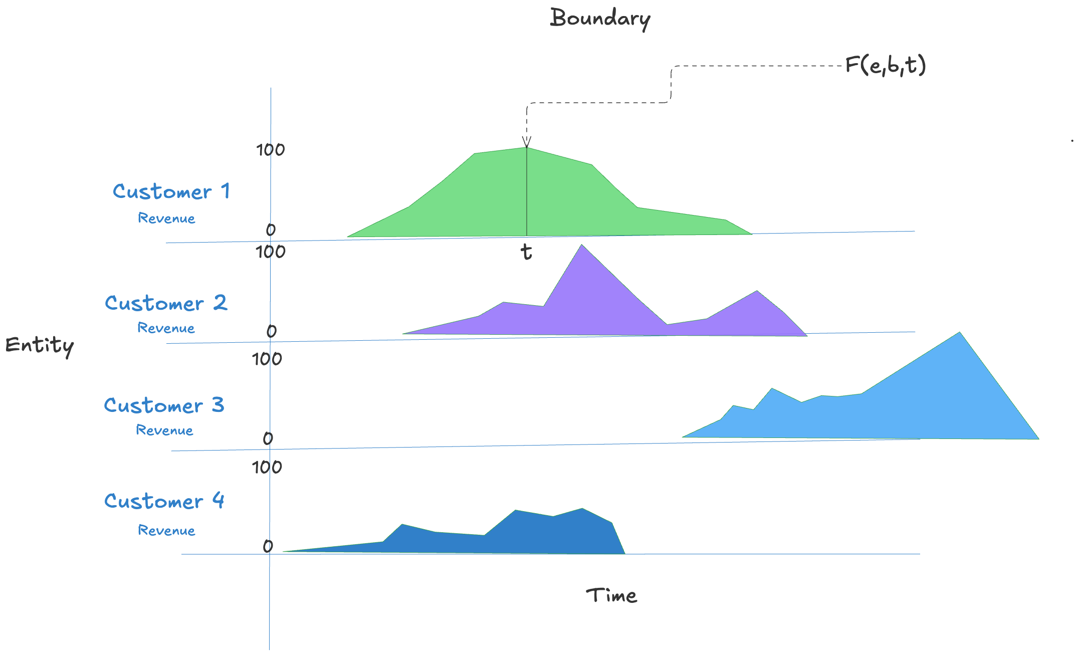
Note that Inside the interval, the value may still drop to zero — presence does not require that every value for the presence function remain greater than zero during the interval.
Here are more examples of presence functions in python.
Note that constant_presence corresponds to the most commonly assumed form of
presence in classical models. It represents entities with uniform presence
over a finite interval—from the start of the event to its end—with constant
instantaneous mass.
Much of queueing theory and flow analysis is based solely on this simple model, where presence is modeled as a rectangular pulse with finite duration and constant density.
The presence calculus generalizes this by allowing arbitrary real-valued functions with compact support over the extended real line $\overline{\mathbb{R}}$, enabling richer modeling of non-uniform, delayed, forecasted, or probabilistic presences.
# Boolean presence: returns 1.0 within [start, end), 0.0 elsewhere
def constant_presence(start: float, end: float) -> PresenceFunction:
    def f(e, b, t):
        return 1.0 if start <= t < end else 0.0
    return f

# Ramped presence: increases linearly from 0.0 to 1.0 over [start, end)
def ramp_presence(start: float, end: float) -> PresenceFunction:
    def f(e, b, t):
        if start <= t < end:
            return (t - start) / (end - start)
        return 0.0
    return f

# Delayed pulse: returns fixed value only after a delay from start
def delayed_presence(start: float, end: float, delay: float = 1.0) -> PresenceFunction:
    def f(e, b, t):
        if start + delay <= t < end:
            return 1.0
        return 0.0
    return f
These functions form the foundation of presence semantics.
Presence functions are defined in the domain and serve as the bridge between discrete
domain events and continuous presence intervals used in the presence calculus.
They are exposed to the presence calculus via the PresenceProtocol.
361@runtime_checkable
362class PresenceProtocol(Protocol):
363    """
364    The PresenceProtocol represents the  contract between an arbitrary presence function
365    and the foo
366    """
367
368    def __call__(self, t0: float, t1: float) -> float: ...
369
370
371
372    def overlaps(self, t0: float, t1: float) -> bool: ...
373
374    @property
375    def onset_time(self) -> float: ...
376
377    @property
378    def reset_time(self) -> float: ...
The PresenceProtocol represents the contract between an arbitrary presence function and the foo
1953def _no_init_or_replace_init(self, *args, **kwargs):
1954    cls = type(self)
1955
1956    if cls._is_protocol:
1957        raise TypeError('Protocols cannot be instantiated')
1958
1959    # Already using a custom `__init__`. No need to calculate correct
1960    # `__init__` to call. This can lead to RecursionError. See bpo-45121.
1961    if cls.__init__ is not _no_init_or_replace_init:
1962        return
1963
1964    # Initially, `__init__` of a protocol subclass is set to `_no_init_or_replace_init`.
1965    # The first instantiation of the subclass will call `_no_init_or_replace_init` which
1966    # searches for a proper new `__init__` in the MRO. The new `__init__`
1967    # replaces the subclass' old `__init__` (ie `_no_init_or_replace_init`). Subsequent
1968    # instantiation of the protocol subclass will thus use the new
1969    # `__init__` and no longer call `_no_init_or_replace_init`.
1970    for base in cls.__mro__:
1971        init = base.__dict__.get('__init__', _no_init_or_replace_init)
1972        if init is not _no_init_or_replace_init:
1973            cls.__init__ = init
1974            break
1975    else:
1976        # should not happen
1977        cls.__init__ = object.__init__
1978
1979    cls.__init__(self, *args, **kwargs)
372 def overlaps(self, t0: float, t1: float) -> bool: ...
381@dataclass(frozen=True)
382class PresenceAssertion:
383    """
384
385    This is the fundamental, immutable construct of The presence calculus,
386    and asserts the presence of an element at a boundary over a continuous interval of time.
387
388    A presence is defined over a half-open interval $[t_0, t_1)$ on the real
389    line, where $t_0$ is the onset time and $t_1$ is the reset time.
390
391    The
392    following constraints must hold:
393
394    - $t_0 < t_1$
395    - $t_0 \\in \\mathbb{R} \\cup \\{-\\infty\\}$
396    - $t_1 \\in \\mathbb{R} \\cup \\{+\\infty\\}$
397    - $t_0 \\ne +\\infty$
398    - $t_1 \\ne -\\infty$
399
400    These rules ensure that the interval is well-formed, bounded on the left,
401    and open on the right. Intervals such as $[2.0, 5.0)$, $[-\\infty, 4.2)$,
402    and $[1.0, +\\infty)$ are allowed, as are the special case $[-\\infty,
403    +\\infty)$ and $[0,0),$ the empty presence.
404
405    With the empty presence as the only exception, intervals with zero or negative duration, or with reversed or
406    undefined bounds, are disallowed.
407    """
408    element: Optional[EntityProtocol]
409    boundary: Optional[EntityProtocol]
410    onset_time: float
411    reset_time: float
412    presence: Optional[PresenceProtocol] = None
413    observer: Optional[EntityProtocol] | str = "observed"
414    assert_time: Optional[float] = 0.0
415
416    def __post_init__(self):
417        """
418        Validates the temporal bounds of the presence interval
419        """
420        if self.onset_time >= self.reset_time:
421            if not (self.onset_time == self.reset_time == 0):
422                raise ValueError(
423                    f"Invalid interval: onset_time ({self.onset_time}) must be less than reset_time ({self.reset_time})")
424
425        if self.onset_time == float("inf"):
426            raise ValueError("Presence cannot begin at +inf")
427
428        if self.reset_time == float("-inf"):
429            raise ValueError("Presence cannot end at -inf")
430
431    def overlaps(self, t0: float, t1: float) -> bool:
432        return self.reset_time > t0 and self.onset_time < t1
433
434    def mass(self) -> float:
435        """
436        Returns the mass of the presence.
437
438
439
440        """
441        onset = max(0.0, self.onset_time)
442        return max(0.0, self.reset_time - onset)
443
444    def mass_contribution(self, t0: float, t1: float) -> float:
445        if t0 >= t1 or not self.overlaps(t0, t1):
446            return 0.0
447        start = max(self.onset_time, t0)
448        end = min(self.reset_time, t1)
449        return max(0.0, end - start)
450
451    def __str__(self) -> str:
452        element_str = str(self.element) if self.element is not None else "None"
453        boundary_str = str(self.boundary) if self.boundary is not None else "None"
454        interval_str = f"[{self.onset_time}, {self.reset_time})"
455        return (
456            f"Presence(element={element_str}, boundary={boundary_str}, "
457            f"interval={interval_str}, provenance={self.observer})"
458        )
This is the fundamental, immutable construct of The presence calculus, and asserts the presence of an element at a boundary over a continuous interval of time.
A presence is defined over a half-open interval $[t_0, t_1)$ on the real line, where $t_0$ is the onset time and $t_1$ is the reset time.
The following constraints must hold:
- $t_0 < t_1$
- $t_0 \in \mathbb{R} \cup {-\infty}$
- $t_1 \in \mathbb{R} \cup {+\infty}$
- $t_0 \ne +\infty$
- $t_1 \ne -\infty$
These rules ensure that the interval is well-formed, bounded on the left, and open on the right. Intervals such as $[2.0, 5.0)$, $[-\infty, 4.2)$, and $[1.0, +\infty)$ are allowed, as are the special case $[-\infty, +\infty)$ and $[0,0),$ the empty presence.
With the empty presence as the only exception, intervals with zero or negative duration, or with reversed or undefined bounds, are disallowed.