pcalc
The Presence Calculus Toolkit
© 2025 Dr. Krishna Kumar SPDX-License-Identifier: MIT
Introduction
The Presence Calculus provides a mathematical formalism for reasoning about the relationship between measures on elements and boundaries in a domain over time.
It begins with the concept of a Presence—a measure over the real numbers, associated with a particular Element (thing) in a domain, observed within a Boundary (place), over a continuous interval of time.
Both Elements and Boundaries belong to an underlying domain $D$ under analysis.
Measure theory offers a general mechanism for representing both presence and its effects. This lets us model concepts such as value, impact, delay, cost, revenue, and user experience as forms of presence. It also enables rigorous reasoning about temporal constructs like time value, delayed value, and the option value of presence.
The Presence Calculus is built on rigorous mathematical foundations— measure theory and topology—anchored by presence as an epistemic primitive.
This frames each presence as an observation made by a specific observer at a specific time, within an open-world setting across an infinite timeline. It enables meaningful reasoning about complex systems where noise, delay, ambiguity, and the provenance of observations play a critical role.
Given a set of presence assertions over a domain $D$, the calculus provides rigorously defined primitives and constructs for analyzing element timelines and trajectories, presence-induced topologies on $D$, and the effects of co-presence—simultaneous element presence—within and across boundaries.#233
These techniques apply consistently across a wide range of domains, including stochastic, non-linear, adaptive, and complex systems.

Motivation
Our primary goal in developing the Presence Calculus is to support rigorous modeling and principled decision-making in complex, real-world domains. We aim to ensure that the use of data in such decisions rests on a foundation that is mathematically precise, logically coherent, and epistemically grounded.
The current state of measurement—particularly in messy, complex domains—is often deficient in all three of these areas. The Presence Calculus emerged from a search for better structural tools in contexts where traditional statistical or causal methods fall short.
Presence Calculus builds on ideas from measure theory and topology, and connects it stochastic process dynamics, queueing theory, and complex systems science—yet remains philosophically distinct from each of them in its focus. This allows it to connect disparate fields while re-framing their perspectives through the common epistemic lens of presence.
The foundational constructs of Presence Calculus allow us to define derived notions such as flow, stability, equilibrium, and coherence precisely, and to relate them to practically useful measures like delay, cost, revenue, and user experience—once interpreted within the semantics of the domain being modeled.
In messy, real-world domains, relationships between elements, boundaries, flows, and effects often emerge from complex, higher-dimensional interactions among many parameters. These patterns are often more amenable to machine analysis in high-dimensional representations than through the simplified, low-dimensional models we typically use to make decisions. The Presence Calculus lets us build such representations, starting from simple, declarative models of presence.
While we illustrate our ideas using real-world decision problems, our focus is not on prescribing what decisions to make or how to make them. That belongs to the application domain of Presence Calculus—a domain we believe is vast.
Our goal is to make this framework accessible enough for others to build powerful applications on top of it, without requiring a deep background in the underlying mathematics (though it will help in following some of the more technical arguments)
The Toolkit
The Presence Calculus Toolkit is a computationally efficient implementation of the core concepts and calculations in presence calculus.
This pcalc module in particular, is an elementary and accessible entry point to some of the more abstract
concepts in the presence calculus. It is a computational model for the calculus
capable of powering real-time analysis and simulation of complex systems. The module is designed as a lightweight,
easy-to-integrate analytical middleware library that connects real-time event streams, simulation models,
and static datasets from a domain to rich visualization and analysis tools.
While we'll provide several examples of end-to-end integrations, the library is open source under the MIT license, and you are encouraged to create models and applications—both commercial and non-commercial—that build on the concepts.
If you are comfortable learning by reading code and implementing models and don't mind just a tiny bit of formal mathematical notation, this is a better entry point to the presence calculus for you.
More background and general, informal discussion around these topics can be found on The Polaris Flow Dispatch.
Reading these docs
The documentation is organized so that you can get a very good idea of the scope of the presence calculus and it's implementation by reading the topics listed on the "submodules" left hand menu, in order.
Each module links to detailed API documentation that is also directly accessible from this page. The index is also searchable once you get familiar with the concepts.
We believe the space of potential applications is vast, and invite you to explore it—and to reach out if you have questions or would like to collaborate with me on helping develop it further.
  1# -*- coding: utf-8 -*-
  2# Copyright (c) 2025 Krishna Kumar
  3# SPDX-License-Identifier: MIT
  4
  5"""
  6#The Presence Calculus Toolkit
  7© 2025 Dr. Krishna Kumar
  8SPDX-License-Identifier: MIT
  9
 10## Introduction
 11
 12The Presence Calculus provides a mathematical formalism for reasoning about
 13the relationship between measures on *elements* and *boundaries* in a domain over *time*.
 14
 15It begins with the concept of a Presence—a measure over the real numbers, associated with
 16a particular *Element* (thing) in a domain, observed within a *Boundary* (place),
 17over a continuous interval of time.
 18
 19Both Elements and Boundaries belong
 20to an underlying domain $D$ under analysis.
 21
 22Measure theory offers a general mechanism for representing
 23both presence and its effects. This lets us model concepts such as value,
 24impact, delay, cost, revenue, and user experience as forms of presence.
 25It also enables rigorous reasoning about temporal constructs like time value,
 26delayed value, and the option value of presence.
 27
 28The Presence Calculus is built on rigorous mathematical foundations—
 29measure theory and topology—anchored by presence as an epistemic primitive.
 30
 31This frames each presence as an observation made by a specific observer
 32at a specific time, within an open-world setting across an infinite timeline.
 33It enables meaningful reasoning about complex systems where
 34noise, delay, ambiguity, and the provenance of observations play a critical role.
 35
 36Given a set of presence assertions over a domain $D$, the calculus provides
 37rigorously defined primitives and constructs for analyzing element timelines
 38and trajectories, presence-induced topologies on $D$, and the effects of
 39co-presence—simultaneous element presence—within and across boundaries.#233
 40
 41
 42These techniques apply consistently across a wide range of domains, including
 43stochastic, non-linear, adaptive, and complex systems.
 44
 45<div style="text-align: center; margin:2em">
 46  <img src="../assets/pcalc/presence_calculus.svg" width="600px" />
 47  <div style="font-size: 0.9em; color: #555; margin-top: 1em; margin-bottom: 1em;">
 48    Figure 1: Key constructs—presences, element paths, presence matrix, and co-presence topology
 49  </div>
 50</div>
 51
 52## Motivation
 53Our primary goal in developing the Presence Calculus is to support rigorous
 54modeling and principled decision-making in complex, real-world domains. We aim
 55to ensure that the use of data in such decisions rests on a foundation that is
 56mathematically precise, logically coherent, and epistemically grounded.
 57
 58The current state of measurement—particularly in messy, complex domains—is often
 59deficient in all three of these areas. The Presence Calculus emerged from a
 60search for better structural tools in contexts where traditional statistical or
 61causal methods fall short.
 62
 63Presence Calculus builds on ideas from measure theory and topology, and
 64connects it stochastic process dynamics, queueing
 65theory, and complex systems science—yet remains philosophically
 66distinct from each of them in its focus. This allows it to connect disparate fields while
 67re-framing their perspectives through the common epistemic lens of presence.
 68
 69The foundational constructs of Presence Calculus allow us to define derived
 70notions such as flow, stability, equilibrium, and coherence precisely, and to
 71relate them to practically useful measures like delay, cost, revenue, and user
 72experience—once interpreted within the semantics of the domain being modeled.
 73
 74In messy, real-world domains, relationships between elements, boundaries, flows,
 75and effects often emerge from complex, higher-dimensional interactions among
 76many parameters. These patterns are often more amenable to machine analysis in
 77high-dimensional representations than through the simplified, low-dimensional
 78models we typically use to make decisions. The Presence Calculus lets us
 79build such representations, starting from simple, declarative models of presence.
 80
 81While we illustrate our ideas using real-world decision problems, our focus is
 82not on prescribing what decisions to make or how to make them. That belongs to
 83the application domain of Presence Calculus—a domain we believe is vast.
 84
 85Our goal is to make this framework accessible enough for others to build powerful
 86applications on top of it, without requiring a deep background in the
 87underlying mathematics (though it will help in following some of the more technical
 88arguments)
 89
 90## The Toolkit
 91
 92The Presence Calculus Toolkit is a computationally efficient implementation of the core concepts and
 93calculations in presence calculus.
 94
 95This `pcalc` module in particular, is an elementary and accessible entry point to some of the more abstract
 96concepts in the presence calculus. It is a computational model for the calculus
 97capable of powering real-time analysis and simulation of complex systems. The module is designed as a lightweight,
 98easy-to-integrate analytical middleware library that connects real-time event streams, simulation models,
 99and static datasets from a domain to rich visualization and analysis tools.
100
101While we'll provide several examples of end-to-end integrations, the library is
102open source under the MIT license, and you are encouraged to create models and
103applications—both commercial and non-commercial—that build on the concepts.
104
105If you are comfortable learning by
106reading code and implementing models and don't mind just a tiny bit of
107formal mathematical notation, this is a better entry point to the presence calculus for you.
108
109More background and general, informal discussion around these topics
110can be found on [The Polaris Flow Dispatch.](https://wwww.polaris-flow-dispatch.com)
111
112## Reading these docs
113
114The documentation is organized so that you can get a very good idea of the
115scope of the presence calculus and it's implementation by reading the
116topics listed on the "submodules" left hand menu, in order.
117
118Each module
119links to detailed API documentation that is also directly accessible from this page.
120The index is also searchable once you get familiar with the concepts.
121
122We believe the space of potential
123applications is vast, and invite you to explore it—and to reach out if you
124have questions or would like to collaborate with me on helping develop it further.
125
126
127[Dr. Krishna Kumar](https://www.linkedin.com/in/krishnaku1/),
128<br> [The Polaris Advisor Program](https://github.com/polarisadvisor)
129
130
131"""
132
133from .entity import Entity, EntityProtocol
134from .presence import PresenceAssertion
135from .time_model import TimeModel
136from .basis_topology import BasisTopology
137from .presence_invariant import PresenceInvariant
138from .presence_matrix import PresenceMatrix
139from .time_scale import Timescale
140from .presence_map import PresenceMap
141from .presence_invariant_discrete import PresenceInvariantDiscrete
142
143__all__ = [
144    # Domain API
145    "entity",
146    Entity, EntityProtocol,
147
148    "presence",
149    PresenceAssertion,
150
151    # Continuous Time Models
152    "time_model",
153    TimeModel,
154    "basis_topology",
155    BasisTopology,
156    "presence_invariant",
157    PresenceInvariant,
158
159    # Discrete Time Models
160    "time_scale",
161    Timescale,
162    "presence_map",
163    PresenceMap,
164    "presence_matrix",
165    PresenceMatrix,
166    "presence_invariant_discrete",
167    PresenceInvariantDiscrete,
168]
220class Entity(EntityMixin, EntityProtocol):
221    """A default implementation of fully functional entity.
222
223    ```python
224    elements = [
225        Entity(id="cust-001", name="Alice Chen", metadata={"type": "customer"}),
226        Entity(id="cust-002", name="Bob Gupta", metadata={"type": "customer"}),
227        Entity(id="pros-003", name="Dana Rivera", metadata={"type": "prospect"}),
228    ]
229    boundaries = [
230        Entity(id="seg-enterprise", name="Enterprise Segment", metadata={"region": "NA"}),
231        Entity(id="seg-smb", name="SMB Segment", metadata={"region": "EMEA"}),
232        Entity(id="seg-dormant", name="Flight Risk", metadata={"status": "inactive", "last login": "2024-06-01"}),
233        Entity(id="seg-prospect", name="Active Prospects", metadata={"status": "demo given"})
234    ]
235
236    for e in elements:
237        print(f"Element: {e.summary()}")
238
239    for b in boundaries:
240        print(f"Boundary: {b.summary()}")
241    ```
242    """
243    __slots__ = ("_id", "_name", "_metadata")
244
245    # noinspection PyProtocol
246    def __init__(self, id: Optional[str] = None, name: Optional[str] = None, metadata: Optional[Dict[str, Any]] = None):
247        self._id: str = id or str(uuid.uuid4())
248        self._name: str = name or self.id
249        self._metadata: Dict[str, Any] = metadata or {}
250
251    @property
252    def id(self) -> str:
253        return self._id
254
255    # noinspection PyProtocol
256    @property
257    def name(self) -> str:
258        return self._name
259
260    @name.setter
261    def name(self, name: str) -> None:
262        self._name = name
263
264    @property
265    def metadata(self) -> Dict[str, Any]:
266        return self._metadata
267
268    def __str__(self) -> str:
269        return self.summary()
A default implementation of fully functional entity.
elements = [
    Entity(id="cust-001", name="Alice Chen", metadata={"type": "customer"}),
    Entity(id="cust-002", name="Bob Gupta", metadata={"type": "customer"}),
    Entity(id="pros-003", name="Dana Rivera", metadata={"type": "prospect"}),
]
boundaries = [
    Entity(id="seg-enterprise", name="Enterprise Segment", metadata={"region": "NA"}),
    Entity(id="seg-smb", name="SMB Segment", metadata={"region": "EMEA"}),
    Entity(id="seg-dormant", name="Flight Risk", metadata={"status": "inactive", "last login": "2024-06-01"}),
    Entity(id="seg-prospect", name="Active Prospects", metadata={"status": "demo given"})
]

for e in elements:
    print(f"Element: {e.summary()}")

for b in boundaries:
    print(f"Boundary: {b.summary()}")
A stable, unique identifier for the entity. Used for indexing and identity. Defaults to a uuid.uuid4().
Inherited Members
105@runtime_checkable
106class EntityProtocol(Protocol):
107    """
108    The interface contract for a domain entity to participate in a presence assertion.
109
110    Each entity requires only a unique identifier, a user-facing name.
111
112    Optional metadata may be provided and exposes specific attributes of the domain
113    entities that are relevant when interpreting or manipulating the results
114    of an analysis using the machinery of the calculus.
115
116    See `Entity` for an example of a concrete implementation.
117    """
118    __init__ = None  # type: ignore
119
120    @property
121    def id(self) -> str:
122        """
123        A stable, unique identifier for the entity.
124        Used for indexing and identity.
125        Defaults to a uuid.uuid4().
126        """
127        ...
128
129    @property
130    def name(self) -> str:
131        """
132        A user facing name for the entity, defaults to the id if None.
133        """
134        ...
135
136    @name.setter
137    def name(self, name: str) -> None:
138        """Setter for name"""
139        ...
140
141    @property
142    def metadata(self) -> Dict[str, Any]:
143        """
144        Optional extensible key-value metadata.
145        """
146        ...
The interface contract for a domain entity to participate in a presence assertion.
Each entity requires only a unique identifier, a user-facing name.
Optional metadata may be provided and exposes specific attributes of the domain entities that are relevant when interpreting or manipulating the results of an analysis using the machinery of the calculus.
See Entity for an example of a concrete implementation.
120    @property
121    def id(self) -> str:
122        """
123        A stable, unique identifier for the entity.
124        Used for indexing and identity.
125        Defaults to a uuid.uuid4().
126        """
127        ...
A stable, unique identifier for the entity. Used for indexing and identity. Defaults to a uuid.uuid4().
381@dataclass(frozen=True)
382class PresenceAssertion:
383    """
384
385    This is the fundamental, immutable construct of The presence calculus,
386    and asserts the presence of an element at a boundary over a continuous interval of time.
387
388    A presence is defined over a half-open interval $[t_0, t_1)$ on the real
389    line, where $t_0$ is the onset time and $t_1$ is the reset time.
390
391    The
392    following constraints must hold:
393
394    - $t_0 < t_1$
395    - $t_0 \\in \\mathbb{R} \\cup \\{-\\infty\\}$
396    - $t_1 \\in \\mathbb{R} \\cup \\{+\\infty\\}$
397    - $t_0 \\ne +\\infty$
398    - $t_1 \\ne -\\infty$
399
400    These rules ensure that the interval is well-formed, bounded on the left,
401    and open on the right. Intervals such as $[2.0, 5.0)$, $[-\\infty, 4.2)$,
402    and $[1.0, +\\infty)$ are allowed, as are the special case $[-\\infty,
403    +\\infty)$ and $[0,0),$ the empty presence.
404
405    With the empty presence as the only exception, intervals with zero or negative duration, or with reversed or
406    undefined bounds, are disallowed.
407    """
408    element: Optional[EntityProtocol]
409    boundary: Optional[EntityProtocol]
410    onset_time: float
411    reset_time: float
412    presence: Optional[PresenceProtocol] = None
413    observer: Optional[EntityProtocol] | str = "observed"
414    assert_time: Optional[float] = 0.0
415
416    def __post_init__(self):
417        """
418        Validates the temporal bounds of the presence interval
419        """
420        if self.onset_time >= self.reset_time:
421            if not (self.onset_time == self.reset_time == 0):
422                raise ValueError(
423                    f"Invalid interval: onset_time ({self.onset_time}) must be less than reset_time ({self.reset_time})")
424
425        if self.onset_time == float("inf"):
426            raise ValueError("Presence cannot begin at +inf")
427
428        if self.reset_time == float("-inf"):
429            raise ValueError("Presence cannot end at -inf")
430
431    def overlaps(self, t0: float, t1: float) -> bool:
432        return self.reset_time > t0 and self.onset_time < t1
433
434    def mass(self) -> float:
435        """
436        Returns the mass of the presence.
437
438
439
440        """
441        onset = max(0.0, self.onset_time)
442        return max(0.0, self.reset_time - onset)
443
444    def mass_contribution(self, t0: float, t1: float) -> float:
445        if t0 >= t1 or not self.overlaps(t0, t1):
446            return 0.0
447        start = max(self.onset_time, t0)
448        end = min(self.reset_time, t1)
449        return max(0.0, end - start)
450
451    def __str__(self) -> str:
452        element_str = str(self.element) if self.element is not None else "None"
453        boundary_str = str(self.boundary) if self.boundary is not None else "None"
454        interval_str = f"[{self.onset_time}, {self.reset_time})"
455        return (
456            f"Presence(element={element_str}, boundary={boundary_str}, "
457            f"interval={interval_str}, provenance={self.observer})"
458        )
This is the fundamental, immutable construct of The presence calculus, and asserts the presence of an element at a boundary over a continuous interval of time.
A presence is defined over a half-open interval $[t_0, t_1)$ on the real line, where $t_0$ is the onset time and $t_1$ is the reset time.
The following constraints must hold:
- $t_0 < t_1$
- $t_0 \in \mathbb{R} \cup {-\infty}$
- $t_1 \in \mathbb{R} \cup {+\infty}$
- $t_0 \ne +\infty$
- $t_1 \ne -\infty$
These rules ensure that the interval is well-formed, bounded on the left, and open on the right. Intervals such as $[2.0, 5.0)$, $[-\infty, 4.2)$, and $[1.0, +\infty)$ are allowed, as are the special case $[-\infty, +\infty)$ and $[0,0),$ the empty presence.
With the empty presence as the only exception, intervals with zero or negative duration, or with reversed or undefined bounds, are disallowed.
 76class TimeModel:
 77
 78
 79    def __init__(self, origin: datetime, unit: CalendarUnit = "seconds"):
 80        self.origin = origin
 81        self.unit = unit
 82
 83    def to_float(self, t: datetime) -> float:
 84        delta = t - self.origin
 85        seconds = delta.total_seconds()
 86
 87        if self.unit == "seconds":
 88            return seconds
 89        if self.unit == "minutes":
 90            return seconds / 60.0
 91        if self.unit == "hours":
 92            return seconds / 3600.0
 93        if self.unit == "days":
 94            return delta.days + (delta.seconds / 86400.0)
 95        if self.unit == "months":
 96            return self._months_between(self.origin, t)
 97        if self.unit == "quarters":
 98            return self._months_between(self.origin, t) / 3.0
 99        if self.unit == "years":
100            return self._months_between(self.origin, t) / 12.0
101
102        raise ValueError(f"Unsupported time unit: {self.unit}")
103
104    def from_float(self, t: float) -> datetime:
105        if self.unit == "seconds":
106            return self.origin + timedelta(seconds=t)
107        if self.unit == "minutes":
108            return self.origin + timedelta(minutes=t)
109        if self.unit == "hours":
110            return self.origin + timedelta(hours=t)
111        if self.unit == "days":
112            return self.origin + timedelta(days=t)
113        if self.unit in {"months", "quarters", "years"}:
114            months = {
115                "months": int(round(t)),
116                "quarters": int(round(t * 3)),
117                "years": int(round(t * 12)),
118            }[self.unit]
119            return self.origin + relativedelta(months=+months)
120
121        raise ValueError(f"Unsupported time unit: {self.unit}")
122
123    @staticmethod
124    def _months_between(d1: datetime, d2: datetime) -> float:
125        """Return the number of calendar months between two dates, fractional."""
126        rd = relativedelta(d2, d1)
127        return rd.years * 12 + rd.months + (rd.days / 30.0)
 83    def to_float(self, t: datetime) -> float:
 84        delta = t - self.origin
 85        seconds = delta.total_seconds()
 86
 87        if self.unit == "seconds":
 88            return seconds
 89        if self.unit == "minutes":
 90            return seconds / 60.0
 91        if self.unit == "hours":
 92            return seconds / 3600.0
 93        if self.unit == "days":
 94            return delta.days + (delta.seconds / 86400.0)
 95        if self.unit == "months":
 96            return self._months_between(self.origin, t)
 97        if self.unit == "quarters":
 98            return self._months_between(self.origin, t) / 3.0
 99        if self.unit == "years":
100            return self._months_between(self.origin, t) / 12.0
101
102        raise ValueError(f"Unsupported time unit: {self.unit}")
104    def from_float(self, t: float) -> datetime:
105        if self.unit == "seconds":
106            return self.origin + timedelta(seconds=t)
107        if self.unit == "minutes":
108            return self.origin + timedelta(minutes=t)
109        if self.unit == "hours":
110            return self.origin + timedelta(hours=t)
111        if self.unit == "days":
112            return self.origin + timedelta(days=t)
113        if self.unit in {"months", "quarters", "years"}:
114            months = {
115                "months": int(round(t)),
116                "quarters": int(round(t * 3)),
117                "years": int(round(t * 12)),
118            }[self.unit]
119            return self.origin + relativedelta(months=+months)
120
121        raise ValueError(f"Unsupported time unit: {self.unit}")
 79class BasisTopology:
 80    """
 81    The foundational topology generated by a set of presence assertions.
 82
 83    Presences are treated as basis elements defining basic open sets.
 84    Internally, presences are grouped into sorted open covers per (element, boundary)
 85    and exposed through join, closure, and overlap operations.
 86    """
 87
 88    def __init__(self, presences: Iterable[PresenceAssertion]) -> None:
 89        """
 90        Initializes the topology from a set of presences.
 91
 92        Internally maintains a SortedSet for each (element, boundary) pair,
 93        ordered by onset_time for efficient merge and overlap operations.
 94        """
 95        self.cover_index: dict[Tuple, SortedSet[PresenceAssertion]] = defaultdict(
 96            lambda: SortedSet(key=presence_sort_key)
 97        )
 98
 99        for p in presences:
100            key = (p.element, p.boundary)
101            self.cover_index[key].add(p)
102
103    def get_cover(self, element, boundary) -> SortedSet[PresenceAssertion]:
104        """
105        Returns the open cover for a given (element, boundary) pair.
106        """
107        return self.cover_index.get((element, boundary), SortedSet(key=presence_sort_key))
108
109    @staticmethod
110    def join(p1: PresenceAssertion, p2: PresenceAssertion) -> PresenceAssertion:
111        """
112        Returns the join of two basis elements if they overlap or touch in time.
113        Returns EMPTY_PRESENCE if the presences are disjoint or incompatible.
114        """
115        if (p1.element, p1.boundary) != (p2.element, p2.boundary):
116            return EMPTY_PRESENCE
117
118        if p1.reset_time < p2.onset_time != float("-inf") and p1.reset_time != float("inf"):
119            return EMPTY_PRESENCE
120        if p2.reset_time < p1.onset_time != float("-inf") and p2.reset_time != float("inf"):
121            return EMPTY_PRESENCE
122
123        return PresenceAssertion(
124            element=p1.element,
125            boundary=p1.boundary,
126            onset_time=min(p1.onset_time, p2.onset_time),
127            reset_time=max(p1.reset_time, p2.reset_time),
128            observer="join",
129        )
130
131    def closure(self) -> set[PresenceAssertion]:
132        """
133        Computes the closure under join for each cover.
134
135        Returns a deduplicated set of merged presences that cover the same regions
136        as the original topology, but without adjacent overlaps.
137        """
138        closed = set()
139
140        for key, cover in self.cover_index.items():
141            merged_cover = []
142            for p in cover:
143                if not merged_cover:
144                    merged_cover.append(p)
145                    continue
146
147                last = merged_cover[-1]
148                j = self.join(last, p)
149
150                if j is not EMPTY_PRESENCE:
151                    merged_cover[-1] = j
152                else:
153                    merged_cover.append(p)
154
155            closed.update(merged_cover)
156
157        return closed
158
159    def find_overlapping(self, presence: PresenceAssertion) -> list[PresenceAssertion]:
160        """
161        Finds all presences in the same cover that overlap with the given presence.
162
163        This is a linear scan from the first potentially overlapping point onward,
164        relying on the sorted order of onset_time.
165        """
166        key = (presence.element, presence.boundary)
167        cover = self.cover_index.get(key, SortedSet(key=presence_sort_key))
168        overlapping = []
169
170        for p in cover.irange(minimum=None, maximum=None):
171            if p.onset_time >= presence.reset_time:
172                break
173            if p.reset_time > presence.onset_time:
174                overlapping.append(p)
175
176        return overlapping
177
178    def __iter__(self):
179        for cover in self.cover_index.values():
180            yield from cover
The foundational topology generated by a set of presence assertions.
Presences are treated as basis elements defining basic open sets. Internally, presences are grouped into sorted open covers per (element, boundary) and exposed through join, closure, and overlap operations.
 88    def __init__(self, presences: Iterable[PresenceAssertion]) -> None:
 89        """
 90        Initializes the topology from a set of presences.
 91
 92        Internally maintains a SortedSet for each (element, boundary) pair,
 93        ordered by onset_time for efficient merge and overlap operations.
 94        """
 95        self.cover_index: dict[Tuple, SortedSet[PresenceAssertion]] = defaultdict(
 96            lambda: SortedSet(key=presence_sort_key)
 97        )
 98
 99        for p in presences:
100            key = (p.element, p.boundary)
101            self.cover_index[key].add(p)
Initializes the topology from a set of presences.
Internally maintains a SortedSet for each (element, boundary) pair, ordered by onset_time for efficient merge and overlap operations.
103    def get_cover(self, element, boundary) -> SortedSet[PresenceAssertion]:
104        """
105        Returns the open cover for a given (element, boundary) pair.
106        """
107        return self.cover_index.get((element, boundary), SortedSet(key=presence_sort_key))
Returns the open cover for a given (element, boundary) pair.
109    @staticmethod
110    def join(p1: PresenceAssertion, p2: PresenceAssertion) -> PresenceAssertion:
111        """
112        Returns the join of two basis elements if they overlap or touch in time.
113        Returns EMPTY_PRESENCE if the presences are disjoint or incompatible.
114        """
115        if (p1.element, p1.boundary) != (p2.element, p2.boundary):
116            return EMPTY_PRESENCE
117
118        if p1.reset_time < p2.onset_time != float("-inf") and p1.reset_time != float("inf"):
119            return EMPTY_PRESENCE
120        if p2.reset_time < p1.onset_time != float("-inf") and p2.reset_time != float("inf"):
121            return EMPTY_PRESENCE
122
123        return PresenceAssertion(
124            element=p1.element,
125            boundary=p1.boundary,
126            onset_time=min(p1.onset_time, p2.onset_time),
127            reset_time=max(p1.reset_time, p2.reset_time),
128            observer="join",
129        )
Returns the join of two basis elements if they overlap or touch in time. Returns EMPTY_PRESENCE if the presences are disjoint or incompatible.
131    def closure(self) -> set[PresenceAssertion]:
132        """
133        Computes the closure under join for each cover.
134
135        Returns a deduplicated set of merged presences that cover the same regions
136        as the original topology, but without adjacent overlaps.
137        """
138        closed = set()
139
140        for key, cover in self.cover_index.items():
141            merged_cover = []
142            for p in cover:
143                if not merged_cover:
144                    merged_cover.append(p)
145                    continue
146
147                last = merged_cover[-1]
148                j = self.join(last, p)
149
150                if j is not EMPTY_PRESENCE:
151                    merged_cover[-1] = j
152                else:
153                    merged_cover.append(p)
154
155            closed.update(merged_cover)
156
157        return closed
Computes the closure under join for each cover.
Returns a deduplicated set of merged presences that cover the same regions as the original topology, but without adjacent overlaps.
159    def find_overlapping(self, presence: PresenceAssertion) -> list[PresenceAssertion]:
160        """
161        Finds all presences in the same cover that overlap with the given presence.
162
163        This is a linear scan from the first potentially overlapping point onward,
164        relying on the sorted order of onset_time.
165        """
166        key = (presence.element, presence.boundary)
167        cover = self.cover_index.get(key, SortedSet(key=presence_sort_key))
168        overlapping = []
169
170        for p in cover.irange(minimum=None, maximum=None):
171            if p.onset_time >= presence.reset_time:
172                break
173            if p.reset_time > presence.onset_time:
174                overlapping.append(p)
175
176        return overlapping
Finds all presences in the same cover that overlap with the given presence.
This is a linear scan from the first potentially overlapping point onward, relying on the sorted order of onset_time.
11class PresenceInvariant:
12    """
13    Computes the components of the Presence Invariant directly from a BasisTopology.
14
15    This invariant expresses a local conservation law of presence mass over any finite
16    time interval [t0, t1), using only the closure of the topology.
17    """
18
19    def __init__(self, topology: BasisTopology):
20        self.topology = topology
21        self.closed_presences = topology.closure()
22
23    def _filter_window(self, t0: float, t1: float) -> list[PresenceAssertion]:
24        return [
25            p for p in self.closed_presences
26            if p.overlaps(t0,t1)
27        ]
28
29    def get_presence_summary(self, t0: float, t1: float) -> Tuple[float, int, float]:
30        """
31        Computes:
32        - Total presence mass A
33        - Number of overlapping presences N
34        - Interval length T
35        """
36        if t0 >= t1:
37            return 0.0, 0, 0.0
38
39        A = 0.0
40        N = 0
41        T = t1 - t0
42
43        for p in self._filter_window(t0, t1):
44            r = p.mass_contribution(t0, t1)
45            if r > 0.0:
46                A += r
47                N += 1
48
49        return A, N, T
50
51    def avg_presence_density(self, t0: float, t1: float) -> float:
52        A, _, T = self.get_presence_summary(t0, t1)
53        return A / T if T > 0 else 0.0
54
55    def incidence_rate(self, t0: float, t1: float) -> float:
56        _, N, T = self.get_presence_summary(t0, t1)
57        return N / T if T > 0 else 0.0
58
59
60    def avg_presence_mass(self, t0: float, t1: float) -> float:
61        A, N, _ = self.get_presence_summary(t0, t1)
62        return A / N if N > 0 else 0.0
63
64    def invariant(self, t0: float, t1: float) -> Tuple[float, float, float]:
65        """
66        Returns:
67            (avg_presence_density, incidence_rate, avg_presence_mass)
68
69        These satisfy the Presence Invariant:
70            avg_presence_density = incidence_rate × avg_presence_mass
71        """
72        A, N, T = self.get_presence_summary(t0, t1)
73        L = A / T if T > 0 else 0.0
74        Λ = N / T if T > 0 else 0.0
75        w = A / N if N > 0 else 0.0
76        return L, Λ, w
Computes the components of the Presence Invariant directly from a BasisTopology.
This invariant expresses a local conservation law of presence mass over any finite time interval [t0, t1), using only the closure of the topology.
29    def get_presence_summary(self, t0: float, t1: float) -> Tuple[float, int, float]:
30        """
31        Computes:
32        - Total presence mass A
33        - Number of overlapping presences N
34        - Interval length T
35        """
36        if t0 >= t1:
37            return 0.0, 0, 0.0
38
39        A = 0.0
40        N = 0
41        T = t1 - t0
42
43        for p in self._filter_window(t0, t1):
44            r = p.mass_contribution(t0, t1)
45            if r > 0.0:
46                A += r
47                N += 1
48
49        return A, N, T
Computes:
- Total presence mass A
- Number of overlapping presences N
- Interval length T
64    def invariant(self, t0: float, t1: float) -> Tuple[float, float, float]:
65        """
66        Returns:
67            (avg_presence_density, incidence_rate, avg_presence_mass)
68
69        These satisfy the Presence Invariant:
70            avg_presence_density = incidence_rate × avg_presence_mass
71        """
72        A, N, T = self.get_presence_summary(t0, t1)
73        L = A / T if T > 0 else 0.0
74        Λ = N / T if T > 0 else 0.0
75        w = A / N if N > 0 else 0.0
76        return L, Λ, w
Returns:
(avg_presence_density, incidence_rate, avg_presence_mass)
These satisfy the Presence Invariant:
avg_presence_density = incidence_rate × avg_presence_mass
 13@dataclass
 14class Timescale:
 15    """
 16    Timescale represents a partitioning of a continuous time interval [t0, t1)
 17    into N = ceil((t1 - t0) / bin_width) contiguous, left-aligned, non-overlapping bins.
 18
 19    Each bin has width `bin_width` and covers a half-open interval:
 20        Bin k = [t0 + k * bin_width, t0 + (k + 1) * bin_width)
 21
 22    This class provides methods for:
 23    - Mapping real-valued timestamps to discrete bin indices
 24    - Extracting the time boundaries of any bin
 25    - Computing which bins an interval [start, end) overlaps
 26    - Estimating how much of a bin is covered by a given interval
 27
 28    **Boundary Behavior**:
 29    - All bins lie strictly within [t0, t1)
 30    - Any time `t` where t < t0 or t >= t1 is considered **outside** the defined timescale
 31    - bin_index(t) may return an out-of-range index if `t < t0` or `t >= t1`
 32
 33    This class does not perform clipping: it assumes all inputs are in-range unless explicitly clipped by the caller.
 34"""
 35
 36    t0: float
 37    """start time of the interval [t0, t1)"""
 38    t1: float
 39    """end time of the interval [t0, t1)"""
 40
 41    bin_width: float
 42    """Width of each bin"""
 43
 44    @property
 45    def num_bins(self) -> int:
 46        """Return number of bins between t0 and t1."""
 47        return int(np.ceil((self.t1 - self.t0) / self.bin_width))
 48
 49    # Mapping from continuous time to discrete bins.
 50    def bin_index(self, time: float) -> int:
 51        """Purpose:
 52            Map a real-valued timestamp to the index of the bin that contains it.
 53
 54        Contract:
 55            Returns k such that bin_start(k) ≤ time < bin_end(k)
 56            Uses floor() logic — i.e., left-aligned binning
 57            No bounds check: time < t0 may yield negative indices; time ≥ t1 may return out-of-bounds indices
 58            Caller is responsible for ensuring t0 ≤ time < t1 if range enforcement is needed
 59        """
 60        return int(np.floor((time - self.t0) / self.bin_width))
 61
 62    def bin_slice(self, start: float, end: float) -> Tuple[int, int]:
 63        """Return the bin indices [start_bin, end_bin) that overlap the interval [start, end).
 64        Contract:
 65            - Clips the interval [start, end) to [t0, t1) before binning
 66            - Computes:
 67                start_bin = floor((clipped_start - t0) / bin_width)
 68                end_bin   = ceil((clipped_end   - t0) / bin_width)
 69            - Resulting slice [start_bin, end_bin) may be empty if the interval does not overlap the timescale
 70            - start_bin ∈ [0, num_bins)
 71            - end_bin   ∈ [0, num_bins]
 72
 73        """
 74        effective_start = max(start, self.t0)
 75        effective_end = min(end, self.t1)
 76        if effective_start >= effective_end:
 77            return 0, 0
 78        start_bin = int(np.floor((effective_start - self.t0) / self.bin_width))
 79        end_bin = int(np.ceil((effective_end - self.t0) / self.bin_width))
 80        return start_bin, end_bin
 81
 82    def fractional_overlap(self, start: float, end: float, bin_idx: int) -> float:
 83        """Return the fraction of the bin at index `bin_idx` that is covered by the interval [start, end).
 84        Contract:
 85            - Computes how much of bin_idx's interval is covered by [start, end)
 86            - Returns value in [0.0, 1.0] based on normalized overlap over bin width
 87            - Clipped to bin extent: overlaps outside the bin are ignored
 88            - Used to compute partial presence contribution within a bin
 89        """
 90        # Clip to timescale
 91        start = max(start, self.t0)
 92        end = min(end, self.t1)
 93
 94        bin_start = self.bin_start(bin_idx)
 95        bin_end = self.bin_end(bin_idx)
 96
 97        overlap_start = max(start, bin_start)
 98        overlap_end = min(end, bin_end)
 99
100        return max(0.0, overlap_end - overlap_start) / self.bin_width
101
102    # Mapping from discrete bins back to continuous time.
103    def bin_start(self, bin_idx: int) -> float:
104        """Return the start time of a bin given its index.
105        Contract:
106            bin_start(k) = t0 + k * bin_width
107        """
108        return self.t0 + bin_idx * self.bin_width
109
110    def bin_end(self, bin_idx: int) -> float:
111        """Return the end time of a bin given its index.
112        Contract:
113            bin_end(k) = t0 + (k + 1) * bin_width
114        """
115        return self.t0 + (bin_idx + 1) * self.bin_width
116
117    def bin_edges(self) -> np.ndarray:
118        """
119        Return an array of bin edge times from t0 to t1, spaced by bin_width.
120
121        The result has length `num_bins + 1` and is safe against floating-point rounding
122        by capping the range to include exactly the number of bins implied by `num_bins()`.
123
124        Contract:
125        - Returns `num_bins + 1` edge values such that:
126            edges = [t0, t0 + bin_width, ..., t1]
127
128        - Guarantees:
129            bin_start(k) == edges[k]
130            bin_end(k)   == edges[k + 1]
131
132        - Handles floating-point rounding safely:
133            If np.arange overproduces due to rounding, result is trimmed
134            to ensure exactly `num_bins + 1` entries.
135
136        This method defines the canonical bin boundaries used across
137        the presence matrix and all derived metrics.
138
139        Example:
140            Timescale(t0=0.0, t1=10.0, bin_width=2.0).bin_edges()
141            => array([0.0, 2.0, 4.0, 6.0, 8.0, 10.0])
142        """
143        num_edges = self.num_bins + 1
144        edges = np.arange(self.t0, self.t0 + num_edges * self.bin_width, self.bin_width)
145
146        # Ensure exactly num_edges (for safety in rare floating-point cases)
147        if len(edges) > num_edges:
148            edges = edges[:num_edges]
149        return edges
150
151
152    def time_range(self, bin_idx: int) -> Tuple[float, float]:
153        """
154            Return the (start, end) time of a bin.
155            Contract:
156                Returns tuple (bin_start(k), bin_end(k))
157                Matches exactly the continuous interval spanned by the bin
158        """
159        return self.bin_start(bin_idx), self.bin_end(bin_idx)
Timescale represents a partitioning of a continuous time interval [t0, t1) into N = ceil((t1 - t0) / bin_width) contiguous, left-aligned, non-overlapping bins.
Each bin has width bin_width and covers a half-open interval:
Bin k = [t0 + k * bin_width, t0 + (k + 1) * bin_width)
This class provides methods for:
- Mapping real-valued timestamps to discrete bin indices
- Extracting the time boundaries of any bin
- Computing which bins an interval [start, end) overlaps
- Estimating how much of a bin is covered by a given interval
Boundary Behavior:
- All bins lie strictly within [t0, t1)
- Any time
twhere t < t0 or t >= t1 is considered outside the defined timescale - bin_index(t) may return an out-of-range index if
t < t0ort >= t1
This class does not perform clipping: it assumes all inputs are in-range unless explicitly clipped by the caller.
44    @property
45    def num_bins(self) -> int:
46        """Return number of bins between t0 and t1."""
47        return int(np.ceil((self.t1 - self.t0) / self.bin_width))
Return number of bins between t0 and t1.
50    def bin_index(self, time: float) -> int:
51        """Purpose:
52            Map a real-valued timestamp to the index of the bin that contains it.
53
54        Contract:
55            Returns k such that bin_start(k) ≤ time < bin_end(k)
56            Uses floor() logic — i.e., left-aligned binning
57            No bounds check: time < t0 may yield negative indices; time ≥ t1 may return out-of-bounds indices
58            Caller is responsible for ensuring t0 ≤ time < t1 if range enforcement is needed
59        """
60        return int(np.floor((time - self.t0) / self.bin_width))
Purpose:
Map a real-valued timestamp to the index of the bin that contains it.
Contract:
Returns k such that bin_start(k) ≤ time < bin_end(k) Uses floor() logic — i.e., left-aligned binning No bounds check: time < t0 may yield negative indices; time ≥ t1 may return out-of-bounds indices Caller is responsible for ensuring t0 ≤ time < t1 if range enforcement is needed
62    def bin_slice(self, start: float, end: float) -> Tuple[int, int]:
63        """Return the bin indices [start_bin, end_bin) that overlap the interval [start, end).
64        Contract:
65            - Clips the interval [start, end) to [t0, t1) before binning
66            - Computes:
67                start_bin = floor((clipped_start - t0) / bin_width)
68                end_bin   = ceil((clipped_end   - t0) / bin_width)
69            - Resulting slice [start_bin, end_bin) may be empty if the interval does not overlap the timescale
70            - start_bin ∈ [0, num_bins)
71            - end_bin   ∈ [0, num_bins]
72
73        """
74        effective_start = max(start, self.t0)
75        effective_end = min(end, self.t1)
76        if effective_start >= effective_end:
77            return 0, 0
78        start_bin = int(np.floor((effective_start - self.t0) / self.bin_width))
79        end_bin = int(np.ceil((effective_end - self.t0) / self.bin_width))
80        return start_bin, end_bin
Return the bin indices [start_bin, end_bin) that overlap the interval [start, end).
Contract:
- Clips the interval [start, end) to [t0, t1) before binning
- Computes: start_bin = floor((clipped_start - t0) / bin_width) end_bin = ceil((clipped_end - t0) / bin_width)
- Resulting slice [start_bin, end_bin) may be empty if the interval does not overlap the timescale
- start_bin ∈ [0, num_bins)
- end_bin ∈ [0, num_bins]
 82    def fractional_overlap(self, start: float, end: float, bin_idx: int) -> float:
 83        """Return the fraction of the bin at index `bin_idx` that is covered by the interval [start, end).
 84        Contract:
 85            - Computes how much of bin_idx's interval is covered by [start, end)
 86            - Returns value in [0.0, 1.0] based on normalized overlap over bin width
 87            - Clipped to bin extent: overlaps outside the bin are ignored
 88            - Used to compute partial presence contribution within a bin
 89        """
 90        # Clip to timescale
 91        start = max(start, self.t0)
 92        end = min(end, self.t1)
 93
 94        bin_start = self.bin_start(bin_idx)
 95        bin_end = self.bin_end(bin_idx)
 96
 97        overlap_start = max(start, bin_start)
 98        overlap_end = min(end, bin_end)
 99
100        return max(0.0, overlap_end - overlap_start) / self.bin_width
Return the fraction of the bin at index bin_idx that is covered by the interval [start, end).
Contract:
- Computes how much of bin_idx's interval is covered by [start, end)
- Returns value in [0.0, 1.0] based on normalized overlap over bin width
- Clipped to bin extent: overlaps outside the bin are ignored
- Used to compute partial presence contribution within a bin
103    def bin_start(self, bin_idx: int) -> float:
104        """Return the start time of a bin given its index.
105        Contract:
106            bin_start(k) = t0 + k * bin_width
107        """
108        return self.t0 + bin_idx * self.bin_width
Return the start time of a bin given its index.
Contract:
bin_start(k) = t0 + k * bin_width
110    def bin_end(self, bin_idx: int) -> float:
111        """Return the end time of a bin given its index.
112        Contract:
113            bin_end(k) = t0 + (k + 1) * bin_width
114        """
115        return self.t0 + (bin_idx + 1) * self.bin_width
Return the end time of a bin given its index.
Contract:
bin_end(k) = t0 + (k + 1) * bin_width
117    def bin_edges(self) -> np.ndarray:
118        """
119        Return an array of bin edge times from t0 to t1, spaced by bin_width.
120
121        The result has length `num_bins + 1` and is safe against floating-point rounding
122        by capping the range to include exactly the number of bins implied by `num_bins()`.
123
124        Contract:
125        - Returns `num_bins + 1` edge values such that:
126            edges = [t0, t0 + bin_width, ..., t1]
127
128        - Guarantees:
129            bin_start(k) == edges[k]
130            bin_end(k)   == edges[k + 1]
131
132        - Handles floating-point rounding safely:
133            If np.arange overproduces due to rounding, result is trimmed
134            to ensure exactly `num_bins + 1` entries.
135
136        This method defines the canonical bin boundaries used across
137        the presence matrix and all derived metrics.
138
139        Example:
140            Timescale(t0=0.0, t1=10.0, bin_width=2.0).bin_edges()
141            => array([0.0, 2.0, 4.0, 6.0, 8.0, 10.0])
142        """
143        num_edges = self.num_bins + 1
144        edges = np.arange(self.t0, self.t0 + num_edges * self.bin_width, self.bin_width)
145
146        # Ensure exactly num_edges (for safety in rare floating-point cases)
147        if len(edges) > num_edges:
148            edges = edges[:num_edges]
149        return edges
Return an array of bin edge times from t0 to t1, spaced by bin_width.
The result has length num_bins + 1 and is safe against floating-point rounding
by capping the range to include exactly the number of bins implied by num_bins().
Contract:
- Returns
num_bins + 1edge values such that: edges = [t0, t0 + bin_width, ..., t1]
Guarantees: bin_start(k) == edges[k] bin_end(k) == edges[k + 1]
Handles floating-point rounding safely: If np.arange overproduces due to rounding, result is trimmed to ensure exactly
num_bins + 1entries.
This method defines the canonical bin boundaries used across the presence matrix and all derived metrics.
Example:
Timescale(t0=0.0, t1=10.0, bin_width=2.0).bin_edges() => array([0.0, 2.0, 4.0, 6.0, 8.0, 10.0])
152    def time_range(self, bin_idx: int) -> Tuple[float, float]:
153        """
154            Return the (start, end) time of a bin.
155            Contract:
156                Returns tuple (bin_start(k), bin_end(k))
157                Matches exactly the continuous interval spanned by the bin
158        """
159        return self.bin_start(bin_idx), self.bin_end(bin_idx)
Return the (start, end) time of a bin.
Contract:
Returns tuple (bin_start(k), bin_end(k)) Matches exactly the continuous interval spanned by the bin
 15@dataclass
 16class PresenceMap:
 17    """
 18        A PresenceMap maps a continuous presence interval [start, end)
 19        onto a discrete time grid defined by a Timescale.
 20
 21        The result is a bin-aligned representation:
 22        - `start_bin` is the index of the first bin touched
 23        - `end_bin` is the exclusive upper bound (i.e., first bin not touched)
 24        - `start_value` and `end_value` represent fractional presence at the edges
 25        - Bins between `start_bin` and `end_bin` are fully or partially covered
 26
 27        Contract:
 28        - A presence is considered "mapped" if it overlaps the timescale [t0, t1)
 29        - Mapped presences always produce:
 30            start_bin ∈ [0, num_bins)
 31            end_bin   ∈ (start_bin, num_bins]
 32        - The bin range [start_bin, end_bin) contains all and only the bins the presence overlaps
 33        - start_value ∈ (0.0, 1.0] if partially covers `start_bin`
 34        - end_value   ∈ (0.0, 1.0] if partially covers `end_bin - 1`
 35    """
 36
 37    presence: PresenceAssertion
 38    """The presence entry"""
 39    time_scale: Timescale
 40    """The time scale that the presence is mapped to"""
 41
 42    is_mapped: bool
 43    """True if the presence has a valid mapping. Unmapped presences have value=-1
 44    for start_slice, end_slice, start_value and end_value.
 45    """
 46
 47    start_bin: int
 48    """The starting bin in the discrete mapping"""
 49    end_bin: int
 50    """The ending bin in the discrete mapping`
 51    of row `row`.
 52    """
 53    start_value: float
 54    """A presence value 0 < p < 1.0 that represents a potentially partial presence at the start of the mapping"""
 55    end_value: float
 56    """A presence value 0 < p < 1.0 that represents a potentially partial presence at the end of the mapping"""
 57
 58    @property
 59    def bin_range(self) -> range:
 60        return range(self.start_bin, self.end_bin) if self.is_mapped else range(0)
 61
 62    @property
 63    def duration(self) -> float:
 64        return self.presence.reset_time - self.presence.onset_time
 65
 66
 67    def __init__(self, presence: PresenceAssertion, time_scale: Timescale):
 68        """
 69        Map a presence interval to matrix slice indices and edge fractional values
 70        using the provided Timescale object.
 71         """
 72        self.presence = presence
 73        self.time_scale = time_scale
 74        ts = self.time_scale
 75        is_mapped = False
 76        start_bin = -1
 77        end_bin = -1
 78        start_value = -1.0
 79        end_value = -1.0
 80
 81        if presence.overlaps(ts.t0, ts.t1):
 82            is_mapped = True
 83            start_bin, end_bin = ts.bin_slice(presence.onset_time, presence.reset_time)
 84            start_value, end_value = self._compute_fractional_values(presence.onset_time, start_bin, presence.reset_time, end_bin)
 85
 86        self.is_mapped = is_mapped
 87        self.start_bin = start_bin
 88        self.end_bin = end_bin
 89        self.start_value = start_value
 90        self.end_value = end_value
 91
 92    def _compute_fractional_values(self, start_time: float, start_bin: int, end_time: float, end_bin: int):
 93        ts = self.time_scale
 94        # Compute partial overlap at start bin
 95        start_value = ts.fractional_overlap(start_time, end_time, start_bin)
 96
 97        # Compute partial overlap at end bin, if not same as start
 98        if end_bin - 1 > start_bin:
 99            end_value = ts.fractional_overlap(start_time, end_time, end_bin - 1)
100        else:
101            end_value = 0.0
102
103        return start_value, end_value
104
105
106    def is_active(self, start_bin: int, end_bin: int):
107        return end_bin > self.start_bin and start_bin < self.end_bin
108
109    def presence_value_in(self, start_time: float, end_time: float) -> float:
110        """
111        Computes total presence value (in time) within [start_time, end_time),
112        using bin-based approximation logic, clipped to the given interval.
113        """
114        ts = self.time_scale
115        bin_width = ts.bin_width
116
117        start_bin, end_bin = ts.bin_slice(start_time, end_time)
118        if self.is_mapped and self.is_active(start_bin, end_bin):
119            #  Clip window to actual presence bounds
120            effective_start = max(self.presence.onset_time, start_time)
121            effective_end = min(self.presence.reset_time, end_time)
122
123            effective_start_bin, effective_end_bin = ts.bin_slice(effective_start, effective_end)
124
125            if start_time == ts.t0 and end_time == ts.t1:
126                start_value = self.start_value
127                end_value = self.end_value
128            else:
129                start_value, end_value = self._compute_fractional_values(effective_start, effective_start_bin, effective_end, effective_end_bin)
130
131            full_bin_value = max(0, effective_end_bin - effective_start_bin - 2)
132
133            fractional_value = start_value + end_value
134
135            return (full_bin_value + fractional_value) * bin_width
136        else:
137            return 0.0
138
139    @property
140    def presence_value(self) -> float:
141        return self.presence_value_in(self.time_scale.t0, self.time_scale.t1)
A PresenceMap maps a continuous presence interval [start, end) onto a discrete time grid defined by a Timescale.
The result is a bin-aligned representation:
start_binis the index of the first bin touchedend_binis the exclusive upper bound (i.e., first bin not touched)start_valueandend_valuerepresent fractional presence at the edges- Bins between
start_binandend_binare fully or partially covered
Contract:
- A presence is considered "mapped" if it overlaps the timescale [t0, t1)
- Mapped presences always produce: start_bin ∈ [0, num_bins) end_bin ∈ (start_bin, num_bins]
- The bin range [start_bin, end_bin) contains all and only the bins the presence overlaps
- start_value ∈ (0.0, 1.0] if partially covers
start_bin - end_value ∈ (0.0, 1.0] if partially covers
end_bin - 1
67    def __init__(self, presence: PresenceAssertion, time_scale: Timescale):
68        """
69        Map a presence interval to matrix slice indices and edge fractional values
70        using the provided Timescale object.
71         """
72        self.presence = presence
73        self.time_scale = time_scale
74        ts = self.time_scale
75        is_mapped = False
76        start_bin = -1
77        end_bin = -1
78        start_value = -1.0
79        end_value = -1.0
80
81        if presence.overlaps(ts.t0, ts.t1):
82            is_mapped = True
83            start_bin, end_bin = ts.bin_slice(presence.onset_time, presence.reset_time)
84            start_value, end_value = self._compute_fractional_values(presence.onset_time, start_bin, presence.reset_time, end_bin)
85
86        self.is_mapped = is_mapped
87        self.start_bin = start_bin
88        self.end_bin = end_bin
89        self.start_value = start_value
90        self.end_value = end_value
Map a presence interval to matrix slice indices and edge fractional values using the provided Timescale object.
True if the presence has a valid mapping. Unmapped presences have value=-1 for start_slice, end_slice, start_value and end_value.
A presence value 0 < p < 1.0 that represents a potentially partial presence at the start of the mapping
A presence value 0 < p < 1.0 that represents a potentially partial presence at the end of the mapping
109    def presence_value_in(self, start_time: float, end_time: float) -> float:
110        """
111        Computes total presence value (in time) within [start_time, end_time),
112        using bin-based approximation logic, clipped to the given interval.
113        """
114        ts = self.time_scale
115        bin_width = ts.bin_width
116
117        start_bin, end_bin = ts.bin_slice(start_time, end_time)
118        if self.is_mapped and self.is_active(start_bin, end_bin):
119            #  Clip window to actual presence bounds
120            effective_start = max(self.presence.onset_time, start_time)
121            effective_end = min(self.presence.reset_time, end_time)
122
123            effective_start_bin, effective_end_bin = ts.bin_slice(effective_start, effective_end)
124
125            if start_time == ts.t0 and end_time == ts.t1:
126                start_value = self.start_value
127                end_value = self.end_value
128            else:
129                start_value, end_value = self._compute_fractional_values(effective_start, effective_start_bin, effective_end, effective_end_bin)
130
131            full_bin_value = max(0, effective_end_bin - effective_start_bin - 2)
132
133            fractional_value = start_value + end_value
134
135            return (full_bin_value + fractional_value) * bin_width
136        else:
137            return 0.0
Computes total presence value (in time) within [start_time, end_time), using bin-based approximation logic, clipped to the given interval.
 18class PresenceMatrix:
 19    """
 20    A scale-invariant, optionally lazy matrix representation of element presences over discrete time bins.
 21
 22    Each row corresponds to a single `Presence`, and each column represents a discrete time bin defined by a `Timescale`.
 23    The matrix records the degree of presence of each element within a given boundary over time, where each value is a real number in [0.0, 1.0]:
 24    - 1.0 = full presence for the duration of the time bin
 25    - 0.0 = no presence
 26    - values in between represent partial presence due to overlap
 27
 28    The matrix can be computed eagerly via `materialize()` or accessed lazily through NumPy-style slicing.
 29
 30    ### Structure
 31
 32    - **Rows:** Each row corresponds to one `Presence` instance.
 33    - **Columns:** Each column represents a discrete bin of time defined by the `Timescale` (from `t0` to `t1` using `bin_width`).
 34    - The matrix shape is therefore `(len(presences), timescale.num_bins)`.
 35
 36    ### Usage
 37
 38    ```python
 39    from pcalc import PresenceMatrix
 40    from metamodel.timescale import Timescale
 41
 42    # Define a time window with bin width of 1.0
 43    ts = Timescale(t0=0.0, t1=5.0, bin_width=1.0)
 44
 45    # Construct lazily
 46    matrix = PresenceMatrix(presences, time_scale=ts)
 47
 48    # Access entire row
 49    row = matrix[0]  # row 0 as 1D array
 50
 51    # Access single value
 52    value = matrix[2, 3]  # presence at row 2, column 3
 53
 54    # Access slice of row
 55    window = matrix[1, 1:4]  # row 1, columns 1–3
 56
 57    # Access slice of rows
 58    rows = matrix[0:2]  # rows 0 and 1
 59
 60    # Access single column
 61    col = matrix[:, 2]  # all rows at column 2
 62
 63    # Access column block
 64    col_block = matrix[:, 1:4]  # all rows, columns 1–3
 65
 66    # Materialize full matrix (optional)
 67    dense = matrix.materialize()
 68    ```
 69
 70    Features
 71    --------
 72    - Lazy evaluation by default; full matrix computed only if needed
 73    - NumPy-style indexing: supports full rows, row/column slicing, and scalar access
 74    - Precision-preserving: partial bin overlaps are retained in the matrix
 75    - Compatible with matrix operations and flow metric calculations
 76    - Backed by a sparse `PresenceMap`, which stores slice indices and fractional overlaps
 77
 78    Notes
 79    -----
 80    - Use `materialize()` if you want to extract or operate on the full dense matrix
 81    - Use `matrix[i, j]`, `matrix[i, j:k]`, or `matrix[:, j]` for lightweight slicing without allocating the full matrix
 82    - Stepped slicing (e.g., `matrix[::2]`) is not currently supported
 83
 84"""
 85
 86    def __init__(self, presences: List[PresenceAssertion], time_scale: Timescale, materialize=False):
 87        """
 88        Construct a presence matrix from a list of Presences and time window configuration.
 89
 90        Args:
 91            presences: A list of `Presence` instances, one per element of interest.
 92            time_scale: The discrete `Timescale` that the matrix will be normalized to.
 93            materialize: If True, immediately constructs the full backing matrix.
 94                     Otherwise, matrix values will be computed on demand using the sparse presence map.
 95        """
 96
 97        self.presence_matrix: Optional[npt.NDArray[np.float64]] = None
 98        """
 99        A real valued matrix with shape (num_Presences, num_bins).
100        When every presence.start and presence.end are whole numbers every value
101        in the matrix is either 0.0 or 1.0. If they are not whole numbers, the presence
102        is mapped to a number between 0.0 and 1.0 at the start and end (or both), with any
103        intermediate value being 1.0.
104        """
105
106        self.time_scale = time_scale
107        """
108        The time scale of the presence matrix.
109        """
110
111        self.presence_map: List[PresenceMap] = []
112        self.shape = None
113        self.init_presence_map(presences)
114
115        if materialize:
116            self.materialize()
117
118    def init_presence_map(self, presences: List[PresenceAssertion]) -> None:
119        """
120        Initialize the internal presence matrix based on the Presence intervals and binning scheme.
121        Only presences that overlap the timescale endpoints [t0, t1) are mapped.
122        """
123        ts = self.time_scale  # Timescale object: includes t0, t1, bin_width
124
125        for row, presence in enumerate(presences):
126            presence_map = PresenceMap(presence, ts)
127            if presence_map.is_mapped:
128                self.presence_map.append(presence_map)
129
130        num_bins = ts.num_bins
131        num_rows = len(self.presence_map)
132        self.shape = (num_rows, num_bins)
133
134    def is_materialized(self) -> bool:
135        """Return True if the backing matrix has been materialized."""
136        return self.presence_matrix is not None
137
138    def materialize(self) -> npt.NDArray[np.float64]:
139        """
140        Materialize and return the full presence matrix from presence maps.
141        If already materialized, this is a no-op and returns the cached matrix.
142
143        Use this only if want the full matrix to operate on. For most cases, you should
144        be able to work with the sparse representation with the presence map and using
145        array slicing on the matrix object. So think twice about why you are materializing
146        a matrix.
147
148        Returns:
149            The dense presence matrix of shape (num_presences, num_bins).
150        """
151        if self.is_materialized():
152            return self.presence_matrix
153
154        num_rows, num_cols = self.shape
155        matrix = np.zeros((num_rows, num_cols), dtype=float)
156
157        for row, pm in enumerate(self.presence_map):
158            if not pm.is_mapped:
159                continue
160            start = pm.start_bin
161            end = pm.end_bin
162            matrix[row, start] = pm.start_value
163            if end - 1 > start:
164                matrix[row, end - 1] = pm.end_value
165            if end - start > 2:
166                matrix[row, start + 1: end - 1] = 1.0
167
168        self.presence_matrix = matrix
169        return self.presence_matrix
170
171    def drop_materialization(self) -> None:
172        """Discard the cached matrix, returning to sparse-only mode."""
173        self.presence_matrix = None
174
175    def _compute_row_slice(self, row: int, start: int, stop: int) -> np.ndarray:
176        """
177        On-demand computation of a row slice from presence map.
178        If the presence is not mapped or out of bounds, returns zeroes.
179        """
180        pm = self.presence_map[row]
181        width = stop - start
182        output = np.zeros(width, dtype=float)
183
184        if not pm.is_mapped:
185            return output
186
187        # Slice and overlap window
188        for col in range(start, stop):
189            if col < pm.start_bin or col >= pm.end_bin:
190                continue
191            elif col == pm.start_bin:
192                output[col - start] = pm.start_value
193            elif col == pm.end_bin - 1:
194                output[col - start] = pm.end_value
195            else:
196                output[col - start] = 1.0
197
198        return output
199
200    @property
201    def presences(self) -> List[PresenceAssertion]:
202        return [pm.presence for pm in self.presence_map]
203
204    def __getitem__(self, index):
205        """
206        Support NumPy-style indexing:
207        - matrix[i]           → row i
208        - matrix[i:j]         → row slice (returns 2D array)
209        - matrix[i, j]        → scalar
210        - matrix[i, j:k]      → row[i], column slice
211        - matrix[:, j]        → column j (all rows)
212        - matrix[:, j:k]      → column block j:k (all rows)
213        """
214        # matrix[i:j] → top-level row slicing
215        if isinstance(index, slice):
216            if index.step is not None:
217                raise ValueError("PresenceMatrix does not support slicing with a step.")
218            start = index.start if index.start is not None else 0
219            stop = index.stop if index.stop is not None else self.shape[0]
220            if self.presence_matrix is not None:
221                return self.presence_matrix[start:stop]
222            return np.array([self[row] for row in range(start, stop)])
223
224        # matrix[i, j], matrix[i, j:k], matrix[:, j]
225        if isinstance(index, tuple):
226            row_idx, col_idx = index
227
228            # matrix[:, j] or matrix[:, j:k]
229            if isinstance(row_idx, slice):
230                if row_idx.step is not None:
231                    raise ValueError("PresenceMatrix does not support stepped row slicing.")
232                row_start = row_idx.start if row_idx.start is not None else 0
233                row_stop = row_idx.stop if row_idx.stop is not None else self.shape[0]
234
235                if isinstance(col_idx, int):
236                    return np.array([self[row, col_idx] for row in range(row_start, row_stop)])
237
238                elif isinstance(col_idx, slice):
239                    if col_idx.step is not None:
240                        raise ValueError("PresenceMatrix does not support stepped column slicing.")
241                    col_start = col_idx.start if col_idx.start is not None else 0
242                    col_stop = col_idx.stop if col_idx.stop is not None else self.shape[1]
243                    return np.array([self[row, col_start:col_stop] for row in range(row_start, row_stop)])
244
245            # matrix[i, j] or matrix[i, j:k]
246            elif isinstance(row_idx, int):
247                if isinstance(col_idx, int):
248                    return self.presence_matrix[row_idx, col_idx] if self.presence_matrix is not None \
249                        else self._compute_row_slice(row_idx, col_idx, col_idx + 1)[0]
250
251                elif isinstance(col_idx, slice):
252                    if col_idx.step is not None:
253                        raise ValueError("PresenceMatrix does not support stepped column slicing.")
254                    start = col_idx.start if col_idx.start is not None else 0
255                    stop = col_idx.stop if col_idx.stop is not None else self.shape[1]
256                    return self.presence_matrix[row_idx, start:stop] if self.presence_matrix is not None \
257                        else self._compute_row_slice(row_idx, start, stop)
258
259        # matrix[i] → single row
260        if isinstance(index, int):
261            return self.presence_matrix[index] if self.presence_matrix is not None \
262                else self._compute_row_slice(index, 0, self.shape[1])
263
264        raise TypeError(f"Invalid index for PresenceMatrix: {index}")
A scale-invariant, optionally lazy matrix representation of element presences over discrete time bins.
Each row corresponds to a single Presence, and each column represents a discrete time bin defined by a Timescale.
The matrix records the degree of presence of each element within a given boundary over time, where each value is a real number in [0.0, 1.0]:
- 1.0 = full presence for the duration of the time bin
- 0.0 = no presence
- values in between represent partial presence due to overlap
The matrix can be computed eagerly via materialize() or accessed lazily through NumPy-style slicing.
Structure
- Rows: Each row corresponds to one
Presenceinstance. - Columns: Each column represents a discrete bin of time defined by the
Timescale(fromt0tot1usingbin_width). - The matrix shape is therefore
(len(presences), timescale.num_bins).
Usage
from pcalc import PresenceMatrix
from metamodel.timescale import Timescale

# Define a time window with bin width of 1.0
ts = Timescale(t0=0.0, t1=5.0, bin_width=1.0)

# Construct lazily
matrix = PresenceMatrix(presences, time_scale=ts)

# Access entire row
row = matrix[0]  # row 0 as 1D array

# Access single value
value = matrix[2, 3]  # presence at row 2, column 3

# Access slice of row
window = matrix[1, 1:4]  # row 1, columns 1–3

# Access slice of rows
rows = matrix[0:2]  # rows 0 and 1

# Access single column
col = matrix[:, 2]  # all rows at column 2

# Access column block
col_block = matrix[:, 1:4]  # all rows, columns 1–3

# Materialize full matrix (optional)
dense = matrix.materialize()
Features
- Lazy evaluation by default; full matrix computed only if needed
- NumPy-style indexing: supports full rows, row/column slicing, and scalar access
- Precision-preserving: partial bin overlaps are retained in the matrix
- Compatible with matrix operations and flow metric calculations
- Backed by a sparse
PresenceMap, which stores slice indices and fractional overlaps
Notes
- Use
materialize()if you want to extract or operate on the full dense matrix - Use
matrix[i, j],matrix[i, j:k], ormatrix[:, j]for lightweight slicing without allocating the full matrix - Stepped slicing (e.g.,
matrix[::2]) is not currently supported
 86    def __init__(self, presences: List[PresenceAssertion], time_scale: Timescale, materialize=False):
 87        """
 88        Construct a presence matrix from a list of Presences and time window configuration.
 89
 90        Args:
 91            presences: A list of `Presence` instances, one per element of interest.
 92            time_scale: The discrete `Timescale` that the matrix will be normalized to.
 93            materialize: If True, immediately constructs the full backing matrix.
 94                     Otherwise, matrix values will be computed on demand using the sparse presence map.
 95        """
 96
 97        self.presence_matrix: Optional[npt.NDArray[np.float64]] = None
 98        """
 99        A real valued matrix with shape (num_Presences, num_bins).
100        When every presence.start and presence.end are whole numbers every value
101        in the matrix is either 0.0 or 1.0. If they are not whole numbers, the presence
102        is mapped to a number between 0.0 and 1.0 at the start and end (or both), with any
103        intermediate value being 1.0.
104        """
105
106        self.time_scale = time_scale
107        """
108        The time scale of the presence matrix.
109        """
110
111        self.presence_map: List[PresenceMap] = []
112        self.shape = None
113        self.init_presence_map(presences)
114
115        if materialize:
116            self.materialize()
Construct a presence matrix from a list of Presences and time window configuration.
Arguments:
- presences: A list of
Presenceinstances, one per element of interest. - time_scale: The discrete
Timescalethat the matrix will be normalized to. - materialize: If True, immediately constructs the full backing matrix. Otherwise, matrix values will be computed on demand using the sparse presence map.
A real valued matrix with shape (num_Presences, num_bins). When every presence.start and presence.end are whole numbers every value in the matrix is either 0.0 or 1.0. If they are not whole numbers, the presence is mapped to a number between 0.0 and 1.0 at the start and end (or both), with any intermediate value being 1.0.
118    def init_presence_map(self, presences: List[PresenceAssertion]) -> None:
119        """
120        Initialize the internal presence matrix based on the Presence intervals and binning scheme.
121        Only presences that overlap the timescale endpoints [t0, t1) are mapped.
122        """
123        ts = self.time_scale  # Timescale object: includes t0, t1, bin_width
124
125        for row, presence in enumerate(presences):
126            presence_map = PresenceMap(presence, ts)
127            if presence_map.is_mapped:
128                self.presence_map.append(presence_map)
129
130        num_bins = ts.num_bins
131        num_rows = len(self.presence_map)
132        self.shape = (num_rows, num_bins)
Initialize the internal presence matrix based on the Presence intervals and binning scheme. Only presences that overlap the timescale endpoints [t0, t1) are mapped.
134    def is_materialized(self) -> bool:
135        """Return True if the backing matrix has been materialized."""
136        return self.presence_matrix is not None
Return True if the backing matrix has been materialized.
138    def materialize(self) -> npt.NDArray[np.float64]:
139        """
140        Materialize and return the full presence matrix from presence maps.
141        If already materialized, this is a no-op and returns the cached matrix.
142
143        Use this only if want the full matrix to operate on. For most cases, you should
144        be able to work with the sparse representation with the presence map and using
145        array slicing on the matrix object. So think twice about why you are materializing
146        a matrix.
147
148        Returns:
149            The dense presence matrix of shape (num_presences, num_bins).
150        """
151        if self.is_materialized():
152            return self.presence_matrix
153
154        num_rows, num_cols = self.shape
155        matrix = np.zeros((num_rows, num_cols), dtype=float)
156
157        for row, pm in enumerate(self.presence_map):
158            if not pm.is_mapped:
159                continue
160            start = pm.start_bin
161            end = pm.end_bin
162            matrix[row, start] = pm.start_value
163            if end - 1 > start:
164                matrix[row, end - 1] = pm.end_value
165            if end - start > 2:
166                matrix[row, start + 1: end - 1] = 1.0
167
168        self.presence_matrix = matrix
169        return self.presence_matrix
Materialize and return the full presence matrix from presence maps. If already materialized, this is a no-op and returns the cached matrix.
Use this only if want the full matrix to operate on. For most cases, you should be able to work with the sparse representation with the presence map and using array slicing on the matrix object. So think twice about why you are materializing a matrix.
Returns:
The dense presence matrix of shape (num_presences, num_bins).
171    def drop_materialization(self) -> None:
172        """Discard the cached matrix, returning to sparse-only mode."""
173        self.presence_matrix = None
Discard the cached matrix, returning to sparse-only mode.
15class PresenceInvariantDiscrete: 16 """ 17 **A finite, scale-invariant, non-equilibrium version of Little's Law.** 18 19 This class computes the components of The Presence Invariant of a presence matrix. 20 21 The Presence Invariant states that for any *finite* interval `[start_time, end_time)` over the timescale `[t0, t1)` 22 of a presence matrix, the following invariant condition holds. 23 24 $$ 25 L = \Lambda \cdot w 26 $$ 27 where 28 29 - **$L$**: the average *presence* per unit time in the interval (see `avg_presence_per_unit_time`). 30 - **$\Lambda$**: The *flow rate* - a finite approximation of *presence arrival/departure rate* (see `flow_rate`). 31 - **$w$**: The *residence time* - a finite approximation of *presence duration* (see `metamodel.presence.Presence.duration`). 32 33 This invariant extends the classical formulation of Little’s Law, an equilibrium-based identity, by establishing a 34 conservation law (of presence) that remains valid across arbitrary timescales, and in non-linear, stochastic processes 35 that operate far from equilibrium. 36 37 It holds unconditionally for any presence matrix and finite window, and serves as a foundational 38 construct for reasoning about flow in non-linear systems. 39 40 The proof of this invariant is surprisingly simple and elementary. 41 42 **Derivation:** 43 44 45 46 Let $A$ be the total presence in the matrix over a finite time window `[start_time, end_time)` of $T$ time units. 47 Let $N$ be the number of distinct presences that overlap the window. 48 49 Let $R(p_i)$ be the portion of the duration of $p_i$ that overlaps the window. This is the *residence time* of $p_i$ in the window. 50 51 The following diagram shows these quantities and the derivation. 52 53 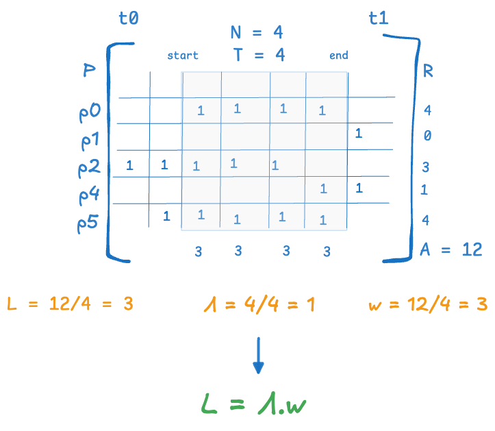 54 55 Then: 56 57 $$ 58 A = \sum_{i=1}^{N} R(p_i) 59 $$ 60 represents the sum of the elements in the presence matrix that foll in the time window `[start_time, end_time)`. 61 62 $A = 12$ presence-time-units in our example. 63 64 Average presence per unit time (see `avg_presence_per_unit_time`) is then: 65 66 $$ 67 L = A/T 68 $$ 69 70 $L = 3$ presences/time-unit in our example. 71 72 $w = $ Average residence time (see `avg_residence_time`) is then: 73 74 $$ 75 w = A/N 76 $$ 77 78 $w=3 time units per presence in our example. 79 80 We will define the flow rate as (see `flow_rate`): 81 82 $$ 83 \Lambda = N/T 84 $$ 85 86 $\Lambda = 1$ presence per time unit in our example. 87 88 Combining these: 89 90 $$ 91 L = A/T = A/N \cdot N/T = N/T \cdot A/N = \Lambda \cdot w 92 $$ 93 94 So we get 95 96 $$ 97 L = \Lambda \cdot w 98 $$ 99 100 101 This identity—what we call the *Presence Invariant*—is equivalent to a fundamental construct used in 102 all proofs of Little’s Law [1], and in particular, to one used by Stidham [2] to give a deterministic 103 proof of Little's Law [3] (see `flow_rate`). 104 105 Both the classical and the current presence-based versions are instances of *Rate Conservation Laws* 106 (as described by Miyazawa [3]). 107 108 However, the conserved quantities differ <sup>[1](#fn1)</sup>: 109 110 - In classical Little’s Law, $L = \lambda \cdot W$ holds *at equilibrium*, using long run arrival/departure rate $\lambda$ and 111 average presence duration $W$. 112 - In the Presence Invariant, $L = \Lambda \cdot w$ holds *universally*, where $\Lambda$ and $w$ are finite window 113 *approximations* of true arrival/departure rate and presence duration. 114 115 Stidham [2] proved the relationship between the quantities in the two versions and showed that 116 the classical form of Little’s Law emerges as a limiting case of the finite-window identity 117 *provided* the system approaches equilibrium as the window grows larger - ie the system is *convergent* in the long run. 118 119 If the system is *divergent* in the long run, at least one of the three quantities grows without limit and 120 the conservation law in the classical version does not hold. 121 122 However, the presence invariant continues to hold regardless of whether the system is convergent or divergent. 123 More details can be found under `flow_rate` and `avg_residence_time`. 124 125 Since non-linear systems rarely reach or maintain equilibrium, the Presence Invariant provides a more robust 126 and widely applicable conservation construct for causal reasoning about flow in such systems. 127 128 <small> 129 <a name="fn1"><strong>[1]</strong></a> 130 Note that we have lowercase $\lambda$ and uppercase $W$ in the classical law, and uppercase $\Lambda$ and 131 lowercase $w$ in the finite-window version, whereas $L$ remains the same in both. 132 133 This reflects the fact that in the Presence Invariant, $\Lambda$ is an overestimate of $\lambda$, and $w$ 134 is an underestimate of $W$. Both identities refer to the *same* observable construct for $L$. 135 </small> 136 137 ## References 138 139 1. **Little’s Law** 140 Little, J. D. C. (2011). *Little’s Law as viewed on its 50th anniversary*. MIT. 141 [https://people.cs.umass.edu/~emery/classes/cmpsci691st/readings/OS/Littles-Law-50-Years-Later.pdf](https://people.cs.umass.edu/~emery/classes/cmpsci691st/readings/OS/Littles-Law-50-Years-Later.pdf) 142 143 2. **Stidham's Proof of Little's Law** 144 Stidham, Shaler. Jr, *A last word on $L = \lambda \cdot W$*.Cornell University. 145 [https://pubsonline.informs.org/doi/epdf/10.1287/opre.22.2.417] 146 147 3. **Miyazawa on Rate Conservation Laws** 148 Miyazawa, M. (1994). *Rate conservation laws: a survey*. Science University of Tokyo. 149 [https://www.rs.tus.ac.jp/miyazawa/pdf-file/Miya1994-QS-RCL.pdf](https://www.rs.tus.ac.jp/miyazawa/pdf-file/Miya1994-QS-RCL.pdf) 150 151 152 """ 153 def __init__(self, matrix: PresenceMatrix): 154 self.matrix = matrix 155 """""" 156 self.presences: list[PresenceAssertion] = matrix.presences 157 """Only presences that overlap the interval [t0, t1) are included in Presence Metrics. 158 Note however that this may include presences that started before the interval or ended after the interval.""" 159 160 self.presence_map: list[PresenceMap] = matrix.presence_map 161 """Only presences that overlap the interval [t0, t1) are included in Presence Metrics. 162 Note however that this may include presences that started before the interval or ended after the interval.""" 163 164 self.ts = matrix.time_scale 165 """The timescale of the presence matrix. This is the default 'window' over which all metrics are computed.""" 166 167 def _resolve_range(self, start_time: Optional[float], end_time: Optional[float]) -> tuple[float, float]: 168 start = start_time if start_time is not None else self.ts.t0 169 end = end_time if end_time is not None else self.ts.t1 170 if start_time < self.ts.t0 or end_time > self.ts.t1: 171 raise ValueError( 172 f"Presence metrics are not defined outside the time scale of the presence matrix." 173 f"Time scale = [{self.ts.t0}, {self.ts.t1})." 174 f"Provided: [{start_time}, {end_time})" 175 ) 176 return start, end 177 178 179 def flow_rate(self, start_time: float = None, end_time: float = None) -> float: 180 """ 181 The flow rate Λ is defined as: 182 number of active presences in the matrix slice [:start_bin:end_bin] / 183 number of time bins in the slice (end_bin - start_bin) 184 185 Conceptually: 186 Let N be the number of presences (rows) that are active (non-zero) 187 in the matrix between start_time and end_time. 188 189 Let T be the number of discrete time bins (columns) in that interval. 190 191 Then: 192 flow_rate = Λ = N / T 193 194 Examples: 195 - If 4 presences span a 6-bin window, flow_rate = 4 / 6 = 0.666... 196 - If only one open-ended presence remains active over a 4-bin window, flow_rate = 1 / 4 = 0.25 197 198 The flow rate is a finite-window estimate of both long-run arrival rate and departure rate. 199 The precise relationship between flow rate, arrival rate, and departure rate is as follows: 200 201 N = number of presences that started *before* start_time (see `starting_presence_count`) 202 + number that started *in* the interval [start_time, end_time) (see `arrival_count`) 203 204 — this is also called the cumulative arrivals into the window 205 206 or equivalently: 207 208 N = number of presences that *ended* in [start_time, end_time) (see `departure_count`) 209 + number that ended *after* end_time (see `ending_presence_count`) 210 211 — this is the departure contribution from the window 212 213 These two decompositions of N are always equal; they just reflect different 214 ways of expressing the same set of active presences. 215 216 Intuitively, over a long enough window, if flow converges, most presences 217 will start and end within the window, with fewer presences that partially overlap 218 the interval at the beginning and end. 219 220 This makes N an (over) estimate of true arrivals or departures over that interval. 221 222 In other words, if flow through the boundary is asymptotically convergent over [start_time, end_time), 223 then: 224 flow_rate → arrival_rate → departure_rate 225 226 When flow is fully convergent over the interval, then: 227 flow_rate = arrival_rate = departure_rate 228 229 This equality is one of the key conditions for *stable* flow through the boundary. 230 231 On the other hand, if flow is not convergent over the interval, the delta between 232 flow rate, arrival rate, and departure rate will be large — either increasing (divergent) 233 or decreasing (convergent) over time. 234 """ 235 _, number_of_presences, num_bins = self.get_presence_summary(start_time, end_time) 236 return number_of_presences/num_bins if num_bins > 0 else 0.0 237 238 def avg_residence_time(self, start_time: float = None, end_time: float = None) -> float: 239 """ 240 Computes the average residence time over the interval [start_time, end_time). 241 242 Let \$ P \$ be the set of presences that overlap the interval \$[\\text{start\\_time}, \\text{end\\_time})\$. 243 244 The *residence time* \$ R(p) \$ is the time that presence \$ p \\in P \$ is active (overlaps) within that interval. 245 246 Presence is computed using bin-weighted overlap, so contributions may be fractional if presences only 247 partially cover a bin. 248 249 The average residence time \$ w \$ is given by: 250 251 \$$ 252 w = \\frac{\\sum_{p \\in P} R(p)}{|P|} 253 \$$ 254 255 If no presences are active in the interval, \$ w = 0.0 \$. 256 257 Note: 258 There are four possible ways a presence can overlap a window [start, end): 259 260 Ticks: 0 1 2 3 4 5 6 7 261 |---|---|---|---|---|---|---| 262 Window: |-----------| 263 264 Case 1: Fully inside 265 [=======] 266 267 Case 2: Starts before, ends inside 268 [=========== 269 270 Case 3: Starts inside, ends after 271 ===========] 272 273 Case 4: Fully spans window 274 [====================] 275 276 In all but Case 1, the window clips the presence, so the residence time 277 is smaller than the presence duration. In Case 1, residence time equals presence duration. 278 279 Intuitively, over a long enough window, if flow converges, most presences 280 will start and end within the window (Case 1), with fewer presences that partially overlap 281 the interval at the beginning and end or span the window (Cases 2–4). 282 283 This makes \$ w \$ an (under)estimate of true presence duration. 284 285 In other words, if flow through the boundary is asymptotically convergent over [start_time, end_time), 286 then: 287 residence time → presence duration. 288 289 When flow is fully convergent over the interval: 290 residence time = presence duration. 291 292 On the other hand, if flow is not convergent over the interval, the delta between 293 residence time and presence duration will be large — either increasing (divergent) 294 or decreasing (convergent) over time. 295 """ 296 total_presence_value, number_of_presences, _ = self.get_presence_summary(start_time, end_time) 297 return total_presence_value / number_of_presences if number_of_presences > 0 else 0.0 298 299 def avg_presence_per_unit_time(self, start_time: float = None, end_time: float = None) -> float: 300 """ 301 Computes the average presence per time bin over the interval [start_time, end_time). 302 303 Let \$ B \$ be the set of discrete time bins that cover the interval \$[\\text{start\\_time}, \\text{end\\_time})\$, 304 and let \$ P(b) \$ denote the total presence across all presences within each bin \$ b \\in B \$. 305 306 The average presence \$ L \$ is given by: 307 308 \$$ 309 L = \\frac{\\sum_{b \\in B} P(b)}{|B|} 310 \$$ 311 312 If the interval spans no bins, \$ L = 0.0 \$. 313 314 Note: 315 This is equivalent to computing the total presence by summing across rows (i.e., sum of all active presence 316 durations we used to compute residence time) divided by the number of bins in the interval. 317 318 Presence is computed using bin-weighted overlap, so contributions may be fractional if presences only 319 partially cover a bin. 320 321 Visually, this corresponds to summing presence *vertically* across bins: 322 323 Example: presences over time bins 324 325 Ticks: 0 1 2 3 4 326 |---|---|---|---| 327 P1: [=======] 328 P2: [=======] 329 P3: [=======] 330 331 Time bin 1: 332 ↑ (bin index 1 = [1, 2)) 333 |---| 334 P1: + 335 P2: + 336 P3: - 337 --------- 338 Sum: 2 339 340 So: 341 - Bin 1 has total presence = 2 342 - If we consider bins 1 to 3 (i.e., [1, 4)), and total presence = 5.5 343 - Then \$ L = 5.5 / 3 = 1.833... \$ 344 345 Conceptually, \$ L \$ reflects the average "load" or concurrency of presence in the system during the interval. 346 347 This metric is the time-relative (per unit time) complements the element-relative residence time \$ w \$. 348 """ 349 total_presence_value, _, num_bins = self.get_presence_summary(start_time, end_time) 350 return total_presence_value / num_bins if num_bins > 0 else 0.0 351 352 def get_presence_summary(self, start_time: float = None, end_time: float = None) -> Tuple[float, float, float]: 353 """ 354 Computes the three core quantities from which all presence-based metrics are derived: 355 356 - Total presence time \$ A \$ over the interval \$[\\text{start\\_time}, \\text{end\\_time})\$ 357 - Number of active presences \$ N \$ (i.e., rows overlapping the interval) 358 - Number of time bins \$ T \$ covering the interval 359 360 These three values form the basis for computing: 361 362 - Average presence per time bin: \$ L = A / T \$ 363 - Average residence time per presence: \$ w = A / N \$ 364 - Flow rate: \$ \\Lambda = N / T \$ 365 366 This method is the common workhorse that underlies `avg_presence_per_time_bin`, 367 `avg_residence_time_per_presence`, and `flow_rate`. 368 369 ... and much of this work lives in `PresenceMap.presence_value_in` 370 """ 371 start, end = self._resolve_range(start_time, end_time) 372 start_bin, end_bin = self.ts.bin_slice(start, end) 373 total_presence_value = 0 374 number_of_presences = 0 375 for pm in self.presence_map: 376 if pm.is_active(start_bin, end_bin): 377 total_presence_value += pm.presence_value_in(start_time, end_time) 378 number_of_presences += 1 379 380 return total_presence_value, number_of_presences, end_bin - start_bin 381 382 def get_presence_metrics(self, start_time: float = None, end_time: float = None) -> Tuple[float, float, float]: 383 """ 384 Computes all three components of the *Presence Invariant* for a finite window 385 $[ \text{start\_time}, \text{end\_time} )$ within the timescale $[ t_0, t_1 )$ 386 of the PresenceMatrix. 387 388 The Presence Invariant states that for *any* such interval: 389 390 $$ 391 L = \Lambda \cdot w 392 $$ 393 394 This invariant holds unconditionally and forms the foundation for reasoning about flow 395 in non-linear systems—systems that often operate far from equilibrium. It generalizes 396 the more familiar equilibrium-based Little’s Law by expressing a conservation law 397 that applies across all time scales. 398 399 - $L$: the *actual* average presence per unit time in the interval (this is not an approximation) 400 - $\Lambda$: the *finite approximation* of presence arrival rate (flow rate) 401 - $w$: the *finite approximation* of presence duration (residence time) 402 403 **Derivation:** 404 405 Let $ A $ be the total presence (i.e., the sum of active elements) in the matrix over the window. 406 Then: 407 408 $$ 409 A = \sum_{\text{rows}} \text{row totals} = \sum_{\text{columns}} \text{column totals} 410 $$ 411 412 Let $ N $ be the number of distinct presences in the window, and $ T $ the window length. 413 414 Then: 415 416 $$ 417 L = \frac{A}{T} = \frac{A}{N} \cdot \frac{N}{T} = w \cdot \Lambda 418 $$ 419 420 Hence: 421 422 $$ 423 L = \Lambda \cdot w 424 $$ 425 426 This identity—what we call the *Presence Invariant*—is a fundamental lemma used in 427 all proofs of Little’s Law [1], and can be seen as its finite-window specialization. 428 429 Both the classical and presence-based versions are instances of *Rate Conservation Laws* 430 (as described by Miyazawa [2]). However, the conserved parameters differ: 431 432 - In classical Little’s Law, $L = \lambda \cdot W$ holds *at equilibrium*, using true arrival rate $\lambda$ and average duration $W$. 433 - In the Presence Invariant, $L = \Lambda \cdot w$ holds *universally*, where $\Lambda$ and $w$ are finite approximations. 434 435 Since non-linear systems rarely reach or maintain equilibrium, the Presence Invariant provides a more robust 436 and widely applicable conservation principle for causal reasoning about flow in such systems. 437 438 ## References 439 440 1. **Little’s Law** 441 Little, J. D. C. (2011). *Little’s Law as viewed on its 50th anniversary*. MIT. 442 [https://people.cs.umass.edu/~emery/classes/cmpsci691st/readings/OS/Littles-Law-50-Years-Later.pdf](https://people.cs.umass.edu/~emery/classes/cmpsci691st/readings/OS/Littles-Law-50-Years-Later.pdf) 443 444 2. **Miyazawa on Rate Conservation Laws** 445 Miyazawa, M. (1994). *Rate conservation laws: a survey*. Science University of Tokyo. 446 [https://www.rs.tus.ac.jp/miyazawa/pdf-file/Miya1994-QS-RCL.pdf](https://www.rs.tus.ac.jp/miyazawa/pdf-file/Miya1994-QS-RCL.pdf) 447 448 """ 449 total_presence_value, number_of_presences, num_bins = self.get_presence_summary(start_time, end_time) 450 451 L = total_presence_value / num_bins if num_bins > 0 else 0.0 452 Λ = number_of_presences / num_bins if num_bins > 0 else 0.0 453 W = total_presence_value / number_of_presences if number_of_presences > 0 else 0.0 454 455 return L, Λ, W 456 457 458 459 460 def starting_presence_count(self, start_time: float = None, end_time: float = None) -> int: 461 start, end = self._resolve_range(start_time, end_time) 462 start_bin, end_bin = self.ts.bin_slice(start, end) 463 464 return sum( 465 1 for pm in self.presence_map 466 if pm.is_active(start_bin, end_bin) 467 #Note: here we must explicitly check the un-clipped 468 # bin indices, since we are looking for end indices that fall outside the 469 # window and even the matrix. So pm.end_bin is not the right test here. 470 and self.ts.bin_index(pm.presence.onset_time) < start_bin 471 ) 472 473 def ending_presence_count(self, start_time: float = None, end_time: float = None) -> int: 474 start, end = self._resolve_range(start_time, end_time) 475 start_bin, end_bin = self.ts.bin_slice(start, end) 476 477 return sum( 478 1 for pm in self.presence_map 479 if pm.is_active(start_bin, end_bin) 480 and (np.isinf(pm.presence.reset_time) or 481 # Note: here we must explicitly check the un-clipped 482 # bin indices, since we are looking for end indices that fall outside the 483 # window and even the matrix. So pm.end_bin is not the right test here. 484 self.ts.bin_index(pm.presence.reset_time) >= end_bin) 485 ) 486 487 def arrival_count(self, start_time: float = None, end_time: float = None) -> int: 488 """The number of presences that started within the window""" 489 start, end = self._resolve_range(start_time, end_time) 490 start_bin, end_bin = self.ts.bin_slice(start, end) 491 492 return sum( 493 1 for pm in self.presence_map 494 if start_bin <= self.ts.bin_index(pm.presence.onset_time) < end_bin 495 ) 496 497 def departure_count(self, start_time: float = None, end_time: float = None) -> int: 498 start, end = self._resolve_range(start_time, end_time) 499 start_bin, end_bin = self.ts.bin_slice(start, end) 500 501 return sum( 502 1 for pm in self.presence_map 503 if np.isfinite(pm.presence.reset_time) 504 and pm.is_active(start_bin, end_bin) 505 and self.ts.bin_index(pm.presence.reset_time) in range(start_bin, end_bin) 506 ) 507 508 509 def foo(self): 510 r""" 511 The key function of this class is to precisely compute the components of key rate conserved quantities 512 tied to Presence under both equilibrium and non-equilibrium conditions. 513 514 The key relationship that matters here is the Presence Invariant, which is rate conservation law 515 for a PresenceMatrix under non-equilibrium condition. 516 517 The Presence Invariant states that for *any* finite interval [start_time, end_time) over the timescale [t0, t1) 518 of a Presence Matrix: 519 520 $$ 521 L = \Lambda \cdot w 522 $$ 523 524 - $L$: the *actual* average presence per unit time in the interval (this is not an approximation) 525 - $\Lambda$: a *finite approximation* of presence arrival rate (flow rate) 526 - $w$: a *finite approximation* of presence duration (residence time) 527 528 This invariant holds unconditionally and forms the foundation for reasoning about flow 529 in non-linear systems—systems that often operate far from equilibrium. It generalizes 530 the more familiar Little’s Law that holds under certain equilibrium conditions as a conservation law 531 that applies across all time scales and non-equilibrium conditions. 532 533 The proof of this invariant is surprisingly simple and elementary. 534 535 **Derivation:** 536 537 Let $ A $ be the total presence (i.e., the sum of active elements) in the matrix over the window. 538 Then: 539 540 $$ 541 A = \sum_{\text{rows}} \text{row totals} = \sum_{\text{columns}} \text{column totals} 542 $$ 543 544 Let $ N $ be the number of distinct presences in the window, and $ T $ the window length. 545 546 Then: 547 548 $$ 549 550 L = \frac{A}{T} = \frac{A}{N} \cdot \frac{N}{T} = w \cdot \Lambda 551 552 $$ 553 554 Hence: 555 556 $$ L = \Lambda \cdot w $$ 557 558 The *Presence Invariant*—is a fundamental lemma used in 559 all proofs of Little’s Law [1], and can be seen as its finite-window version. 560 561 Both the classical and presence-based versions are instances of *Rate Conservation Laws* 562 (as described by Miyazawa [2]). However, the conserved parameters differ: 563 564 - In classical Little’s Law, $L = \lambda \cdot W$ holds *at equilibrium*, using true arrival rate $\lambda$ 565 and average duration $W$. 566 - In the Presence Invariant, $L = \Lambda \cdot w$ holds *universally*, where $\Lambda$ and $w$ are finite 567 window approximations. 568 569 Since non-linear systems rarely reach or maintain equilibrium, the Presence Invariant provides a more robust 570 and widely applicable conservation principle for causal reasoning about flow in such systems. 571 572 References: 573 574 1. **Little’s Law** 575 Little, J. D. C. (2011). *Little’s Law as viewed on its 50th anniversary*. MIT. 576 [https://people.cs.umass.edu/~emery/classes/cmpsci691st/readings/OS/Littles-Law-50-Years-Later.pdf](https://people.cs.umass.edu/~emery/classes/cmpsci691st/readings/OS/Littles-Law-50-Years-Later.pdf) 577 578 2. **Miyazawa on Rate Conservation Laws** 579 Miyazawa, M. (1994). *Rate conservation laws: a survey*. Science University of Tokyo. 580 [https://www.rs.tus.ac.jp/miyazawa/pdf-file/Miya1994-QS-RCL.pdf](https://www.rs.tus.ac.jp/miyazawa/pdf-file/Miya1994-QS-RCL.pdf) 581 """
A finite, scale-invariant, non-equilibrium version of Little's Law.
This class computes the components of The Presence Invariant of a presence matrix.
The Presence Invariant states that for any finite interval [start_time, end_time) over the timescale [t0, t1)
of a presence matrix, the following invariant condition holds.
$$ L = \Lambda \cdot w $$ where
- $L$: the average presence per unit time in the interval (see
avg_presence_per_unit_time). - $\Lambda$: The flow rate - a finite approximation of presence arrival/departure rate (see
flow_rate). - $w$: The residence time - a finite approximation of presence duration (see
metamodel.presence.Presence.duration).
This invariant extends the classical formulation of Little’s Law, an equilibrium-based identity, by establishing a conservation law (of presence) that remains valid across arbitrary timescales, and in non-linear, stochastic processes that operate far from equilibrium.
It holds unconditionally for any presence matrix and finite window, and serves as a foundational construct for reasoning about flow in non-linear systems.
The proof of this invariant is surprisingly simple and elementary.
Derivation:
Let $A$ be the total presence in the matrix over a finite time window [start_time, end_time) of $T$ time units.
Let $N$ be the number of distinct presences that overlap the window.
Let $R(p_i)$ be the portion of the duration of $p_i$ that overlaps the window. This is the residence time of $p_i$ in the window.
The following diagram shows these quantities and the derivation.

Then:
$$
A = \sum_{i=1}^{N} R(p_i)
$$
represents the sum of the elements in the presence matrix that foll in the time window [start_time, end_time).
$A = 12$ presence-time-units in our example.
Average presence per unit time (see avg_presence_per_unit_time) is then:
$$ L = A/T $$
$L = 3$ presences/time-unit in our example.
$w = $ Average residence time (see avg_residence_time) is then:
$$ w = A/N $$
$w=3 time units per presence in our example.
We will define the flow rate as (see flow_rate):
$$ \Lambda = N/T $$
$\Lambda = 1$ presence per time unit in our example.
Combining these:
$$ L = A/T = A/N \cdot N/T = N/T \cdot A/N = \Lambda \cdot w $$
So we get
$$ L = \Lambda \cdot w $$
This identity—what we call the Presence Invariant—is equivalent to a fundamental construct used in
all proofs of Little’s Law [1], and in particular, to one used by Stidham [2] to give a deterministic
proof of Little's Law [3] (see flow_rate).
Both the classical and the current presence-based versions are instances of Rate Conservation Laws (as described by Miyazawa [3]).
However, the conserved quantities differ 1:
- In classical Little’s Law, $L = \lambda \cdot W$ holds at equilibrium, using long run arrival/departure rate $\lambda$ and average presence duration $W$.
- In the Presence Invariant, $L = \Lambda \cdot w$ holds universally, where $\Lambda$ and $w$ are finite window approximations of true arrival/departure rate and presence duration.
Stidham [2] proved the relationship between the quantities in the two versions and showed that the classical form of Little’s Law emerges as a limiting case of the finite-window identity provided the system approaches equilibrium as the window grows larger - ie the system is convergent in the long run.
If the system is divergent in the long run, at least one of the three quantities grows without limit and the conservation law in the classical version does not hold.
However, the presence invariant continues to hold regardless of whether the system is convergent or divergent.
More details can be found under flow_rate and avg_residence_time.
Since non-linear systems rarely reach or maintain equilibrium, the Presence Invariant provides a more robust and widely applicable conservation construct for causal reasoning about flow in such systems.
[1] Note that we have lowercase $\lambda$ and uppercase $W$ in the classical law, and uppercase $\Lambda$ and lowercase $w$ in the finite-window version, whereas $L$ remains the same in both. This reflects the fact that in the Presence Invariant, $\Lambda$ is an overestimate of $\lambda$, and $w$ is an underestimate of $W$. Both identities refer to the same observable construct for $L$.References
Little’s Law Little, J. D. C. (2011). Little’s Law as viewed on its 50th anniversary. MIT. https://people.cs.umass.edu/~emery/classes/cmpsci691st/readings/OS/Littles-Law-50-Years-Later.pdf
Stidham's Proof of Little's Law Stidham, Shaler. Jr, A last word on $L = \lambda \cdot W$.Cornell University. [https://pubsonline.informs.org/doi/epdf/10.1287/opre.22.2.417]
Miyazawa on Rate Conservation Laws Miyazawa, M. (1994). Rate conservation laws: a survey. Science University of Tokyo. https://www.rs.tus.ac.jp/miyazawa/pdf-file/Miya1994-QS-RCL.pdf
153    def __init__(self, matrix: PresenceMatrix):
154        self.matrix = matrix
155        """"""
156        self.presences: list[PresenceAssertion] = matrix.presences
157        """Only presences that overlap the interval [t0, t1) are included in Presence Metrics.
158        Note however that this may include presences that started before the interval or ended after the interval."""
159
160        self.presence_map: list[PresenceMap] = matrix.presence_map
161        """Only presences that overlap the interval [t0, t1) are included in Presence Metrics.
162        Note however that this may include presences that started before the interval or ended after the interval."""
163
164        self.ts = matrix.time_scale
165        """The timescale of the presence matrix. This is the default 'window' over which all metrics are computed."""
Only presences that overlap the interval [t0, t1) are included in Presence Metrics. Note however that this may include presences that started before the interval or ended after the interval.
Only presences that overlap the interval [t0, t1) are included in Presence Metrics. Note however that this may include presences that started before the interval or ended after the interval.
The timescale of the presence matrix. This is the default 'window' over which all metrics are computed.
179    def flow_rate(self, start_time: float = None, end_time: float = None) -> float:
180        """
181        The flow rate Λ is defined as:
182            number of active presences in the matrix slice [:start_bin:end_bin] /
183            number of time bins in the slice (end_bin - start_bin)
184
185        Conceptually:
186            Let N be the number of presences (rows) that are active (non-zero)
187            in the matrix between start_time and end_time.
188
189            Let T be the number of discrete time bins (columns) in that interval.
190
191            Then:
192                flow_rate = Λ = N / T
193
194        Examples:
195            - If 4 presences span a 6-bin window, flow_rate = 4 / 6 = 0.666...
196            - If only one open-ended presence remains active over a 4-bin window, flow_rate = 1 / 4 = 0.25
197
198        The flow rate is a finite-window estimate of both long-run arrival rate and departure rate.
199        The precise relationship between flow rate, arrival rate, and departure rate is as follows:
200
201            N = number of presences that started *before* start_time (see `starting_presence_count`)
202                + number that started *in* the interval [start_time, end_time) (see `arrival_count`)
203
204              — this is also called the cumulative arrivals into the window
205
206            or equivalently:
207
208            N = number of presences that *ended* in [start_time, end_time) (see `departure_count`)
209                + number that ended *after* end_time (see `ending_presence_count`)
210
211              — this is the departure contribution from the window
212
213            These two decompositions of N are always equal; they just reflect different
214            ways of expressing the same set of active presences.
215
216        Intuitively, over a long enough window, if flow converges, most presences
217        will start and end within the window, with fewer presences that partially overlap
218        the interval at the beginning and end.
219
220        This makes N an (over) estimate of true arrivals or departures over that interval.
221
222        In other words, if flow through the boundary is asymptotically convergent over [start_time, end_time),
223        then:
224            flow_rate → arrival_rate → departure_rate
225
226        When flow is fully convergent over the interval, then:
227            flow_rate = arrival_rate = departure_rate
228
229        This equality is one of the key conditions for *stable* flow through the boundary.
230
231        On the other hand, if flow is not convergent over the interval, the delta between
232        flow rate, arrival rate, and departure rate will be large — either increasing (divergent)
233        or decreasing (convergent) over time.
234        """
235        _, number_of_presences, num_bins = self.get_presence_summary(start_time, end_time)
236        return number_of_presences/num_bins if num_bins > 0 else 0.0
The flow rate Λ is defined as: number of active presences in the matrix slice [:start_bin:end_bin] / number of time bins in the slice (end_bin - start_bin)
Conceptually:
Let N be the number of presences (rows) that are active (non-zero) in the matrix between start_time and end_time.
Let T be the number of discrete time bins (columns) in that interval.
Then: flow_rate = Λ = N / T
Examples:
- If 4 presences span a 6-bin window, flow_rate = 4 / 6 = 0.666...
- If only one open-ended presence remains active over a 4-bin window, flow_rate = 1 / 4 = 0.25
The flow rate is a finite-window estimate of both long-run arrival rate and departure rate. The precise relationship between flow rate, arrival rate, and departure rate is as follows:
N = number of presences that started *before* start_time (see `starting_presence_count`)
    + number that started *in* the interval [start_time, end_time) (see `arrival_count`)

  — this is also called the cumulative arrivals into the window

or equivalently:

N = number of presences that *ended* in [start_time, end_time) (see `departure_count`)
    + number that ended *after* end_time (see `ending_presence_count`)

  — this is the departure contribution from the window

These two decompositions of N are always equal; they just reflect different
ways of expressing the same set of active presences.
Intuitively, over a long enough window, if flow converges, most presences will start and end within the window, with fewer presences that partially overlap the interval at the beginning and end.
This makes N an (over) estimate of true arrivals or departures over that interval.
In other words, if flow through the boundary is asymptotically convergent over [start_time, end_time), then: flow_rate → arrival_rate → departure_rate
When flow is fully convergent over the interval, then: flow_rate = arrival_rate = departure_rate
This equality is one of the key conditions for stable flow through the boundary.
On the other hand, if flow is not convergent over the interval, the delta between flow rate, arrival rate, and departure rate will be large — either increasing (divergent) or decreasing (convergent) over time.
238    def avg_residence_time(self, start_time: float = None, end_time: float = None) -> float:
239        """
240            Computes the average residence time over the interval [start_time, end_time).
241
242            Let \$ P \$ be the set of presences that overlap the interval \$[\\text{start\\_time}, \\text{end\\_time})\$.
243
244            The *residence time* \$ R(p) \$ is the time that presence \$ p \\in P \$ is active (overlaps) within that interval.
245
246            Presence is computed using bin-weighted overlap, so contributions may be fractional if presences only
247            partially cover a bin.
248
249            The average residence time \$ w \$ is given by:
250
251            \$$
252            w = \\frac{\\sum_{p \\in P} R(p)}{|P|}
253            \$$
254
255            If no presences are active in the interval, \$ w = 0.0 \$.
256
257            Note:
258                There are four possible ways a presence can overlap a window [start, end):
259
260                Ticks:     0   1   2   3   4   5   6   7
261                           |---|---|---|---|---|---|---|
262                Window:          |-----------|
263
264                Case 1: Fully inside
265                                     [=======]
266
267                Case 2: Starts before, ends inside
268                              [===========
269
270                Case 3: Starts inside, ends after
271                                     ===========]
272
273                Case 4: Fully spans window
274                              [====================]
275
276                In all but Case 1, the window clips the presence, so the residence time
277                is smaller than the presence duration. In Case 1, residence time equals presence duration.
278
279                Intuitively, over a long enough window, if flow converges, most presences
280                will start and end within the window (Case 1), with fewer presences that partially overlap
281                the interval at the beginning and end or span the window (Cases 2–4).
282
283                This makes \$ w \$ an (under)estimate of true presence duration.
284
285                In other words, if flow through the boundary is asymptotically convergent over [start_time, end_time),
286                then:
287                    residence time → presence duration.
288
289                When flow is fully convergent over the interval:
290                    residence time = presence duration.
291
292                On the other hand, if flow is not convergent over the interval, the delta between
293                residence time and presence duration will be large — either increasing (divergent)
294                or decreasing (convergent) over time.
295        """
296        total_presence_value, number_of_presences, _ = self.get_presence_summary(start_time, end_time)
297        return total_presence_value / number_of_presences if number_of_presences > 0 else 0.0
Computes the average residence time over the interval [start_time, end_time).
Let \$ P \$ be the set of presences that overlap the interval \$[\text{start_time}, \text{end_time})\$.
The residence time \$ R(p) \$ is the time that presence \$ p \in P \$ is active (overlaps) within that interval.
Presence is computed using bin-weighted overlap, so contributions may be fractional if presences only partially cover a bin.
The average residence time \$ w \$ is given by:
\$$ w = \frac{\sum_{p \in P} R(p)}{|P|} \$$
If no presences are active in the interval, \$ w = 0.0 \$.
Note:
There are four possible ways a presence can overlap a window [start, end):
Ticks: 0 1 2 3 4 5 6 7 |---|---|---|---|---|---|---| Window: |-----------|
Case 1: Fully inside [=======]
Case 2: Starts before, ends inside [===========
Case 3: Starts inside, ends after ===========]
Case 4: Fully spans window [====================]
In all but Case 1, the window clips the presence, so the residence time is smaller than the presence duration. In Case 1, residence time equals presence duration.
Intuitively, over a long enough window, if flow converges, most presences will start and end within the window (Case 1), with fewer presences that partially overlap the interval at the beginning and end or span the window (Cases 2–4).
This makes \$ w \$ an (under)estimate of true presence duration.
In other words, if flow through the boundary is asymptotically convergent over [start_time, end_time), then: residence time → presence duration.
When flow is fully convergent over the interval: residence time = presence duration.
On the other hand, if flow is not convergent over the interval, the delta between residence time and presence duration will be large — either increasing (divergent) or decreasing (convergent) over time.
299    def avg_presence_per_unit_time(self, start_time: float = None, end_time: float = None) -> float:
300        """
301        Computes the average presence per time bin over the interval [start_time, end_time).
302
303        Let \$ B \$ be the set of discrete time bins that cover the interval \$[\\text{start\\_time}, \\text{end\\_time})\$,
304        and let \$ P(b) \$ denote the total presence across all presences within each bin \$ b \\in B \$.
305
306        The average presence \$ L \$ is given by:
307
308        \$$
309        L = \\frac{\\sum_{b \\in B} P(b)}{|B|}
310        \$$
311
312        If the interval spans no bins, \$ L = 0.0 \$.
313
314        Note:
315            This is equivalent to computing the total presence by summing across rows (i.e., sum of all active presence
316            durations we used to compute residence time) divided by the number of bins in the interval.
317
318            Presence is computed using bin-weighted overlap, so contributions may be fractional if presences only
319            partially cover a bin.
320
321            Visually, this corresponds to summing presence *vertically* across bins:
322
323            Example: presences over time bins
324
325            Ticks:     0   1   2   3   4
326                       |---|---|---|---|
327            P1:         [=======]
328            P2:             [=======]
329            P3:                 [=======]
330
331            Time bin 1:
332                          ↑   (bin index 1 = [1, 2))
333                          |---|
334                      P1:   +
335                      P2:   +
336                      P3:   -
337                    ---------
338                    Sum:     2
339
340            So:
341                - Bin 1 has total presence = 2
342                - If we consider bins 1 to 3 (i.e., [1, 4)), and total presence = 5.5
343                - Then \$ L = 5.5 / 3 = 1.833... \$
344
345            Conceptually, \$ L \$ reflects the average "load" or concurrency of presence in the system during the interval.
346
347            This metric is the time-relative (per unit time) complements the element-relative residence time \$ w \$.
348        """
349        total_presence_value, _, num_bins = self.get_presence_summary(start_time, end_time)
350        return total_presence_value / num_bins if num_bins > 0 else 0.0
Computes the average presence per time bin over the interval [start_time, end_time).
Let \$ B \$ be the set of discrete time bins that cover the interval \$[\text{start_time}, \text{end_time})\$, and let \$ P(b) \$ denote the total presence across all presences within each bin \$ b \in B \$.
The average presence \$ L \$ is given by:
\$$ L = \frac{\sum_{b \in B} P(b)}{|B|} \$$
If the interval spans no bins, \$ L = 0.0 \$.
Note:
This is equivalent to computing the total presence by summing across rows (i.e., sum of all active presence durations we used to compute residence time) divided by the number of bins in the interval.
Presence is computed using bin-weighted overlap, so contributions may be fractional if presences only partially cover a bin.
Visually, this corresponds to summing presence vertically across bins:
Example: presences over time bins
Ticks: 0 1 2 3 4 |---|---|---|---| P1: [=======] P2: [=======] P3: [=======]
Time bin 1: ↑ (bin index 1 = [1, 2)) |---| P1: + P2: + P3: - --------- Sum: 2
So: - Bin 1 has total presence = 2 - If we consider bins 1 to 3 (i.e., [1, 4)), and total presence = 5.5 - Then \$ L = 5.5 / 3 = 1.833... \$
Conceptually, \$ L \$ reflects the average "load" or concurrency of presence in the system during the interval.
This metric is the time-relative (per unit time) complements the element-relative residence time \$ w \$.
352    def get_presence_summary(self, start_time: float = None, end_time: float = None) -> Tuple[float, float, float]:
353        """
354            Computes the three core quantities from which all presence-based metrics are derived:
355
356            - Total presence time \$ A \$ over the interval \$[\\text{start\\_time}, \\text{end\\_time})\$
357            - Number of active presences \$ N \$ (i.e., rows overlapping the interval)
358            - Number of time bins \$ T \$ covering the interval
359
360            These three values form the basis for computing:
361
362            - Average presence per time bin: \$ L = A / T \$
363            - Average residence time per presence: \$ w = A / N \$
364            - Flow rate: \$ \\Lambda = N / T \$
365
366            This method is the common workhorse that underlies `avg_presence_per_time_bin`,
367            `avg_residence_time_per_presence`, and `flow_rate`.
368
369            ... and much of this work lives in `PresenceMap.presence_value_in`
370        """
371        start, end = self._resolve_range(start_time, end_time)
372        start_bin, end_bin = self.ts.bin_slice(start, end)
373        total_presence_value = 0
374        number_of_presences = 0
375        for pm in self.presence_map:
376            if pm.is_active(start_bin, end_bin):
377                total_presence_value += pm.presence_value_in(start_time, end_time)
378                number_of_presences += 1
379
380        return total_presence_value, number_of_presences, end_bin - start_bin
Computes the three core quantities from which all presence-based metrics are derived:
- Total presence time \$ A \$ over the interval \$[\text{start_time}, \text{end_time})\$
- Number of active presences \$ N \$ (i.e., rows overlapping the interval)
- Number of time bins \$ T \$ covering the interval
These three values form the basis for computing:
- Average presence per time bin: \$ L = A / T \$
- Average residence time per presence: \$ w = A / N \$
- Flow rate: \$ \Lambda = N / T \$
This method is the common workhorse that underlies avg_presence_per_time_bin,
avg_residence_time_per_presence, and flow_rate.
... and much of this work lives in PresenceMap.presence_value_in
382    def get_presence_metrics(self, start_time: float = None, end_time: float = None) -> Tuple[float, float, float]:
383        """
384        Computes all three components of the *Presence Invariant* for a finite window
385        $[ \text{start\_time}, \text{end\_time} )$ within the timescale $[ t_0, t_1 )$
386        of the PresenceMatrix.
387
388        The Presence Invariant states that for *any* such interval:
389
390            $$
391            L = \Lambda \cdot w
392            $$
393
394        This invariant holds unconditionally and forms the foundation for reasoning about flow
395        in non-linear systems—systems that often operate far from equilibrium. It generalizes
396        the more familiar equilibrium-based Little’s Law by expressing a conservation law
397        that applies across all time scales.
398
399        - $L$: the *actual* average presence per unit time in the interval (this is not an approximation)
400        - $\Lambda$: the *finite approximation* of presence arrival rate (flow rate)
401        - $w$: the *finite approximation* of presence duration (residence time)
402
403        **Derivation:**
404
405        Let $ A $ be the total presence (i.e., the sum of active elements) in the matrix over the window.
406        Then:
407
408        $$
409        A = \sum_{\text{rows}} \text{row totals} = \sum_{\text{columns}} \text{column totals}
410        $$
411
412        Let $ N $ be the number of distinct presences in the window, and $ T $ the window length.
413
414        Then:
415
416        $$
417        L = \frac{A}{T} = \frac{A}{N} \cdot \frac{N}{T} = w \cdot \Lambda
418        $$
419
420        Hence:
421
422        $$
423        L = \Lambda \cdot w
424        $$
425
426        This identity—what we call the *Presence Invariant*—is a fundamental lemma used in
427        all proofs of Little’s Law [1], and can be seen as its finite-window specialization.
428
429        Both the classical and presence-based versions are instances of *Rate Conservation Laws*
430        (as described by Miyazawa [2]). However, the conserved parameters differ:
431
432        - In classical Little’s Law, $L = \lambda \cdot W$ holds *at equilibrium*, using true arrival rate $\lambda$ and average duration $W$.
433        - In the Presence Invariant, $L = \Lambda \cdot w$ holds *universally*, where $\Lambda$ and $w$ are finite approximations.
434
435        Since non-linear systems rarely reach or maintain equilibrium, the Presence Invariant provides a more robust
436        and widely applicable conservation principle for causal reasoning about flow in such systems.
437
438        ## References
439
440            1. **Little’s Law**
441               Little, J. D. C. (2011). *Little’s Law as viewed on its 50th anniversary*. MIT.
442               [https://people.cs.umass.edu/~emery/classes/cmpsci691st/readings/OS/Littles-Law-50-Years-Later.pdf](https://people.cs.umass.edu/~emery/classes/cmpsci691st/readings/OS/Littles-Law-50-Years-Later.pdf)
443
444            2. **Miyazawa on Rate Conservation Laws**
445               Miyazawa, M. (1994). *Rate conservation laws: a survey*. Science University of Tokyo.
446               [https://www.rs.tus.ac.jp/miyazawa/pdf-file/Miya1994-QS-RCL.pdf](https://www.rs.tus.ac.jp/miyazawa/pdf-file/Miya1994-QS-RCL.pdf)
447
448        """
449        total_presence_value, number_of_presences, num_bins = self.get_presence_summary(start_time, end_time)
450
451        L = total_presence_value / num_bins if num_bins > 0 else 0.0
452        Λ = number_of_presences / num_bins if num_bins > 0 else 0.0
453        W = total_presence_value / number_of_presences if number_of_presences > 0 else 0.0
454
455        return L, Λ, W
Computes all three components of the Presence Invariant for a finite window $[ ext{start_time}, ext{end_time} )$ within the timescale $[ t_0, t_1 )$ of the PresenceMatrix.
The Presence Invariant states that for any such interval:
$$
L = \Lambda \cdot w
$$
This invariant holds unconditionally and forms the foundation for reasoning about flow in non-linear systems—systems that often operate far from equilibrium. It generalizes the more familiar equilibrium-based Little’s Law by expressing a conservation law that applies across all time scales.
- $L$: the actual average presence per unit time in the interval (this is not an approximation)
- $\Lambda$: the finite approximation of presence arrival rate (flow rate)
- $w$: the finite approximation of presence duration (residence time)
Derivation:
Let $ A $ be the total presence (i.e., the sum of active elements) in the matrix over the window. Then:
$$ A = \sum_{ ext{rows}} ext{row totals} = \sum_{ ext{columns}} ext{column totals} $$
Let $ N $ be the number of distinct presences in the window, and $ T $ the window length.
Then:
$$ L = rac{A}{T} = rac{A}{N} \cdot rac{N}{T} = w \cdot \Lambda $$
Hence:
$$ L = \Lambda \cdot w $$
This identity—what we call the Presence Invariant—is a fundamental lemma used in all proofs of Little’s Law [1], and can be seen as its finite-window specialization.
Both the classical and presence-based versions are instances of Rate Conservation Laws (as described by Miyazawa [2]). However, the conserved parameters differ:
- In classical Little’s Law, $L = \lambda \cdot W$ holds at equilibrium, using true arrival rate $\lambda$ and average duration $W$.
- In the Presence Invariant, $L = \Lambda \cdot w$ holds universally, where $\Lambda$ and $w$ are finite approximations.
Since non-linear systems rarely reach or maintain equilibrium, the Presence Invariant provides a more robust and widely applicable conservation principle for causal reasoning about flow in such systems.
References
1. **Little’s Law**
   Little, J. D. C. (2011). *Little’s Law as viewed on its 50th anniversary*. MIT.
   [https://people.cs.umass.edu/~emery/classes/cmpsci691st/readings/OS/Littles-Law-50-Years-Later.pdf](https://people.cs.umass.edu/~emery/classes/cmpsci691st/readings/OS/Littles-Law-50-Years-Later.pdf)

2. **Miyazawa on Rate Conservation Laws**
   Miyazawa, M. (1994). *Rate conservation laws: a survey*. Science University of Tokyo.
   [https://www.rs.tus.ac.jp/miyazawa/pdf-file/Miya1994-QS-RCL.pdf](https://www.rs.tus.ac.jp/miyazawa/pdf-file/Miya1994-QS-RCL.pdf)
460    def starting_presence_count(self, start_time: float = None, end_time: float = None) -> int:
461        start, end = self._resolve_range(start_time, end_time)
462        start_bin, end_bin = self.ts.bin_slice(start, end)
463
464        return sum(
465            1 for pm in self.presence_map
466            if pm.is_active(start_bin, end_bin)
467            #Note: here we must explicitly check the un-clipped
468            # bin indices, since we are looking for end indices that fall outside the
469            # window and even the matrix. So pm.end_bin is not the right test here.
470            and self.ts.bin_index(pm.presence.onset_time) < start_bin
471        )
473    def ending_presence_count(self, start_time: float = None, end_time: float = None) -> int:
474        start, end = self._resolve_range(start_time, end_time)
475        start_bin, end_bin = self.ts.bin_slice(start, end)
476
477        return sum(
478            1 for pm in self.presence_map
479            if pm.is_active(start_bin, end_bin)
480            and (np.isinf(pm.presence.reset_time) or
481                 # Note: here we must explicitly check the un-clipped
482                 # bin indices, since we are looking for end indices that fall outside the
483                 # window and even the matrix. So pm.end_bin is not the right test here.
484                 self.ts.bin_index(pm.presence.reset_time) >= end_bin)
485        )
487    def arrival_count(self, start_time: float = None, end_time: float = None) -> int:
488        """The number of presences that started within the window"""
489        start, end = self._resolve_range(start_time, end_time)
490        start_bin, end_bin = self.ts.bin_slice(start, end)
491
492        return sum(
493            1 for pm in self.presence_map
494            if start_bin <= self.ts.bin_index(pm.presence.onset_time) < end_bin
495        )
The number of presences that started within the window
497    def departure_count(self, start_time: float = None, end_time: float = None) -> int:
498        start, end = self._resolve_range(start_time, end_time)
499        start_bin, end_bin = self.ts.bin_slice(start, end)
500
501        return sum(
502            1 for pm in self.presence_map
503            if np.isfinite(pm.presence.reset_time)
504            and pm.is_active(start_bin, end_bin)
505            and self.ts.bin_index(pm.presence.reset_time) in range(start_bin, end_bin)
506        )
509    def foo(self):
510        r"""
511            The key function of this class is to precisely compute the components of key rate conserved quantities
512            tied to Presence under both equilibrium and non-equilibrium conditions.
513
514            The key relationship that matters here is the Presence Invariant, which is rate conservation law
515            for a PresenceMatrix under non-equilibrium condition.
516
517            The Presence Invariant states that for *any* finite interval [start_time, end_time) over the timescale [t0, t1)
518            of a Presence Matrix:
519
520                    $$
521                    L = \Lambda \cdot w
522                    $$
523
524                - $L$: the *actual* average presence per unit time in the interval (this is not an approximation)
525                - $\Lambda$: a *finite approximation* of presence arrival rate (flow rate)
526                - $w$: a *finite approximation* of presence duration (residence time)
527
528                This invariant holds unconditionally and forms the foundation for reasoning about flow
529                in non-linear systems—systems that often operate far from equilibrium. It generalizes
530                the more familiar Little’s Law that holds under certain equilibrium conditions as a conservation law
531                that applies across all time scales and non-equilibrium conditions.
532
533                The proof of this invariant is surprisingly simple and elementary.
534
535                **Derivation:**
536
537                Let $ A $ be the total presence (i.e., the sum of active elements) in the matrix over the window.
538                Then:
539
540                $$
541                A = \sum_{\text{rows}} \text{row totals} = \sum_{\text{columns}} \text{column totals}
542                $$
543
544                Let $ N $ be the number of distinct presences in the window, and $ T $ the window length.
545
546                Then:
547
548                $$
549
550                L = \frac{A}{T} = \frac{A}{N} \cdot \frac{N}{T} = w \cdot \Lambda
551
552                $$
553
554                Hence:
555
556                $$ L = \Lambda \cdot w $$
557
558                The *Presence Invariant*—is a fundamental lemma used in
559                all proofs of Little’s Law [1], and can be seen as its finite-window version.
560
561                Both the classical and presence-based versions are instances of *Rate Conservation Laws*
562                (as described by Miyazawa [2]). However, the conserved parameters differ:
563
564                - In classical Little’s Law, $L = \lambda \cdot W$ holds *at equilibrium*, using true arrival rate $\lambda$
565                and average duration $W$.
566                - In the Presence Invariant, $L = \Lambda \cdot w$ holds *universally*, where $\Lambda$ and $w$ are finite
567                window approximations.
568
569                Since non-linear systems rarely reach or maintain equilibrium, the Presence Invariant provides a more robust
570                and widely applicable conservation principle for causal reasoning about flow in such systems.
571
572                References:
573
574                1. **Little’s Law**
575                   Little, J. D. C. (2011). *Little’s Law as viewed on its 50th anniversary*. MIT.
576                   [https://people.cs.umass.edu/~emery/classes/cmpsci691st/readings/OS/Littles-Law-50-Years-Later.pdf](https://people.cs.umass.edu/~emery/classes/cmpsci691st/readings/OS/Littles-Law-50-Years-Later.pdf)
577
578                2. **Miyazawa on Rate Conservation Laws**
579                   Miyazawa, M. (1994). *Rate conservation laws: a survey*. Science University of Tokyo.
580                   [https://www.rs.tus.ac.jp/miyazawa/pdf-file/Miya1994-QS-RCL.pdf](https://www.rs.tus.ac.jp/miyazawa/pdf-file/Miya1994-QS-RCL.pdf)
581            """
The key function of this class is to precisely compute the components of key rate conserved quantities tied to Presence under both equilibrium and non-equilibrium conditions.
The key relationship that matters here is the Presence Invariant, which is rate conservation law for a PresenceMatrix under non-equilibrium condition.
The Presence Invariant states that for any finite interval [start_time, end_time) over the timescale [t0, t1) of a Presence Matrix:
    $$
    L = \Lambda \cdot w
    $$

- $L$: the *actual* average presence per unit time in the interval (this is not an approximation)
- $\Lambda$: a *finite approximation* of presence arrival rate (flow rate)
- $w$: a *finite approximation* of presence duration (residence time)

This invariant holds unconditionally and forms the foundation for reasoning about flow
in non-linear systems—systems that often operate far from equilibrium. It generalizes
the more familiar Little’s Law that holds under certain equilibrium conditions as a conservation law
that applies across all time scales and non-equilibrium conditions.

The proof of this invariant is surprisingly simple and elementary.

**Derivation:**

Let $ A $ be the total presence (i.e., the sum of active elements) in the matrix over the window.
Then:

$$
A = \sum_{\text{rows}} \text{row totals} = \sum_{\text{columns}} \text{column totals}
$$

Let $ N $ be the number of distinct presences in the window, and $ T $ the window length.

Then:

$$

L = \frac{A}{T} = \frac{A}{N} \cdot \frac{N}{T} = w \cdot \Lambda

$$

Hence:

$$ L = \Lambda \cdot w $$

The *Presence Invariant*—is a fundamental lemma used in
all proofs of Little’s Law [1], and can be seen as its finite-window version.

Both the classical and presence-based versions are instances of *Rate Conservation Laws*
(as described by Miyazawa [2]). However, the conserved parameters differ:

- In classical Little’s Law, $L = \lambda \cdot W$ holds *at equilibrium*, using true arrival rate $\lambda$
and average duration $W$.
- In the Presence Invariant, $L = \Lambda \cdot w$ holds *universally*, where $\Lambda$ and $w$ are finite
window approximations.

Since non-linear systems rarely reach or maintain equilibrium, the Presence Invariant provides a more robust
and widely applicable conservation principle for causal reasoning about flow in such systems.

References:

1. **Little’s Law**
   Little, J. D. C. (2011). *Little’s Law as viewed on its 50th anniversary*. MIT.
   [https://people.cs.umass.edu/~emery/classes/cmpsci691st/readings/OS/Littles-Law-50-Years-Later.pdf](https://people.cs.umass.edu/~emery/classes/cmpsci691st/readings/OS/Littles-Law-50-Years-Later.pdf)

2. **Miyazawa on Rate Conservation Laws**
   Miyazawa, M. (1994). *Rate conservation laws: a survey*. Science University of Tokyo.
   [https://www.rs.tus.ac.jp/miyazawa/pdf-file/Miya1994-QS-RCL.pdf](https://www.rs.tus.ac.jp/miyazawa/pdf-file/Miya1994-QS-RCL.pdf)